Loboda Igor

Development Of Normal State Model.

Abstract

For a determination of gas turbine technical state many diagnosing techniques analyze in real time the deviations of measured parameters from a normal state model. Above performance degradation a lot of factors influence deeply on these deviations too and diagnosing success depends on model perfection. This paper looks at the process of creation and adjustment of such gaspath parameter model on the base of application of real maintenance data and nonlinear thermodynamic model. The main focus of the work was to find the best model variant for gas turbine monitoring system.

Nomenclature

NSM – normal state model;

 - inlet and control conditions vector;

 - vector of state parameters;

 - gaspath parameters vector;

Gf – fuel consumption;

nFT - free turbine rotation speed;

TH, PH - atmospheric temperature and pressure;

nHP – gas-generator rotation speed;

PC, PT – compressor and turbine pressures;

TC, TT, TFT – temperatures of compressor, turbine, and free turbine;

δYmax, δYmin – maximal and minimal gaspath parameter deviations;

σY – standard gaspath parameter deviation;

t – registration point number.

1. Introduction

Gas turbine component failures, e.g. compressor foiling or combustor distress, cause reduced power and efficiency.

Under typical maintenance regimes gas turbines are washed at regular intervals, for example, every month. It was happened, however, that compressor can become foiled more quickly – for instance, due to increased air pollution. As well as reduced capacity, this can lead to the impossibility of compressor recovery by washing and to the overhaul at high cost.

Improved early failure detection, prediction, and prevention may significantly reduce fuel consumption and life cycle cost for a gas turbine. The techniques based on diagnostic analysis of gaspath measured parameters are widely used for these aims and considered as principal and sufficiently complex elements of gas turbine performance monitoring system.

2. Gas Turbine Performance Monitoring

Automatic monitoring system is an integral part of modern gas turbine power plants and is applied not only for maintenance needs but for aims of gas turbine development and tests too. The algorithms of trend analysis of gas path measured parameters  (gas pressures and temperatures, rotor rotation speeds, fuel consumption …) are able to predict gaspath failures and prognosticate the gas turbine remaining life without turbine shut down and disassembling. Above the gas path, the control system and measurement system may be monitored on these parameters too.

3. Normal State Model

Gaspath parameters depend on functioning regime which is determined by the inlet and control conditions  and gas turbine technical state described by the vector  of state parameters of gas turbine components. That is why any static model of gaspath parameters may be presented in the following general view

.                             (1)

Among static models used in diagnostics the multi-regime nonlinear thermodynamic model is considered as principal and most complex. Mathematically the relation (1) for this model is formed after the solution of the system of algebraic equations reflecting the conditions of components combined work on steady-state regimes.

Let the vector  corresponds to a gas turbine normal state. In this case the dependency

                     (2)

presents a normal state model (NSM) which may be used for the forming of the relative parameter changes (deviations)

 .                          (3)

Theoretically, the deviations  are free of regime influence; therefore they serve as gas turbine degradation indicators and are widely used for technical state estimation, failure detection and prediction [1, 2].

Deviations caused by real failures do not exceed the level of 5%. That is why the total error induced by measurement and model inaccuracy must remain considerably low for correct failure detection; this explains serious metrological requirements to the NSM.

The model accuracy must be kept on constantly low level in every region of argument space (space of possible values of inlet and control conditions ). Otherwise, any change of the functioning regime may produce a significant jump of the deviations which will mask the failure caused trend. Because of this same reason, all factors affecting a turbine behavior must be taken into account in the model.

4. Initial Data, Approach Used

The stationary power plant with free turbine for gas-pump-over-set was chosen as an investigation object. Selecting the NSM structure for this plant we have taken into account the following information.

At first, for this type plant the functioning regime is determined by two control conditions (fuel consumption Gf  and free turbine rotation speed nFT) and two inlet conditions (atmospheric temperature TH and pressure PH ), therefore these four parameters are chosen as model arguments.

At second, it is famous that a function of every gas turbine parameter Yi presents a smooth surface and is well evaluated by polynomials.

At third, the polynomial function of order three and above has an inclination to rapid form change in zones of real data absence for function coefficient determination.

Thus, the following second order polynomial function of four arguments was chosen

   (4)

This function was applied for a description of six gaspath parameters: nHP – gas-generator rotation speed; PC, PT – compressor and turbine pressures; TC, TT, TFT – temperatures of compressor, turbine, and free turbine.

The diagnostic database of the power plant served as a source of maintenance data for a calculation and verification of NSM of the chosen above structure. The database contains registered with one-hour period average numbers of filtered gas turbine parameters. It was important for our work that the registration interval includes the compressor fouling and next washing.

During the NSM investigation on the Matlab (MathWorks, Inc.) different NSM variants were analyzed for consecutive model improvement and every such analysis cycle included the following operations:

·  formation of a learning sample with the parameters  and  from the base for an estimation of NSM coefficients;

·   NSM coefficient calculation by the standard least squares method;

·   formation of a testing sample from the base for a verification of calculated NSM;

·   NSM computation and determination of the deviations (3) in the points of the testing sample;

·   estimation of NSM quality analyzing a behavior and statistical characteristics of the deviations.

Chosen statistical characteristics were: δYmax, δYmin – maximal and minimal deviation numbers; σY – standard deviation. During behavior analysis the principal criteria of NSM perfection were an interference level and a possibility of reliable visual detection of the compressor fouling and washing.

5. Calculations And Result Analysis

Learning sample size and structure were varied in described below calculations and, additionally, an influence of measurement errors was analyzed. The results are discussed on the example of turbine temperature deviation plots for the constant testing sample of 4094 database regime points.

Variant 1. First 100 points of the base were used in the learning sample for the model (4) formation and the deviations (3) were calculated for every point number t of the total testing sample. Presented in the Fig.1 the turbine temperature deviations δTT demonstrate the very great scattering. It may be explained by the fact that all used learning sample registration points are concentrated near one constant turbine regime and the model formed on these points loses the accuracy at other regimes.

Variant 2. The learning sample was formed from 100 points of different gas turbine regimes. Corresponding turbine temperature deviations of the Fig.2 show an evident progress in NSM quality however inexplicable deviation changes are so great that, for example, still exceed the jump caused by the compressor washing near the point number 900. The next step of NSM adjustment was simple and clear - to increase total learning sample size.

Variant 3. The learning sample was created from 694 consecutive points including the points of the variants 1 and 2. For this sample a subsequent model improvement may be noted in the Fig.3.

However, for learning sample increase there is a real restriction related with gas turbine state change with the time. The learning sample has to contain the points of constant turbine state in order to prevent a state influence on the NSM and provide a physical deviation plot.

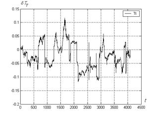
Fig.1. Deviations TT: variant 1

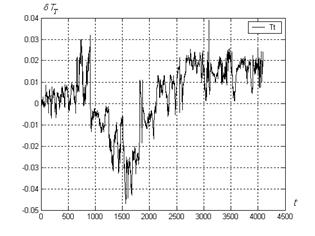
Fig.2. Deviations TT: variant 2

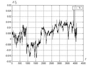
Fig.3. Deviations TT: variant 3

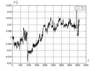
Fig.4. Deviations TT: variant 4

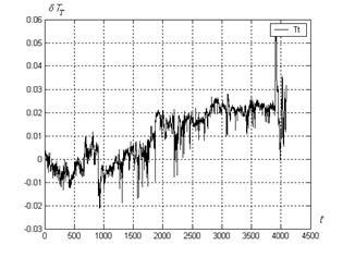
Fig.5. Deviations TT: malfunction of TH sensor

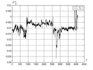
Fig.6. Deviations TC: variant 4

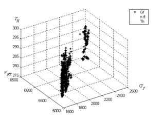
Fig.7. Distribution of maintenance points

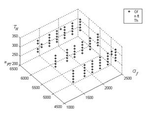
Fig.8. Distribution of thermodynamic model points

So, it is a serious problem to collect maintenance data for sufficiently different conditions  during short gas turbine run-time. For instance, as may be seen in the Fig.7, the variant 3 learning sample points occupy only limited zones of the space “Gf - nFT - TH”.

To overcome this obstacle we have suggested applying the nonlinear thermodynamic model for learning sample generation.

Variant 4. The learning sample included 270 uniformly distributed points (see the Fig.8) generated by the thermodynamic model. The NSM calculated on present sample has very low level of the deviations on this same sample (δYmax = 0.0014, δYmin = - 0.0017, σY = 0.0005) that means a good thermodynamic model description by the NSM and confirms a correct selection of NSM structure. Corresponding testing sample deviations are presented in the Fig.4 which in comparison with the Fig.3 demonstrates further growth of NSM quality in real data description.

Above concerned bad structure of learning sample, other inaccuracy sources were investigated too. For instance, earlier analysis [3] of the deviation jumps near the point 4000 (see Fig.4) has shown that they happen from transient error of TH sensor. Next example: malfunction of other TH sensor produced sharp negative impulses on the deviation curve which are distinguished clearly in the Fig.5 compared with the Fig.4.

The deviations δTC of other monitored parameter – the compressor temperature corresponding to the variant 4 of the learning sample are presented in the Fig.6. Together with the deviations δTT of the Fig.4 they demonstrate achieved model accuracy. It may be seen that the deviations rightly reflect the state of gas turbine but the noise remains relatively high especially in the right part of the plots.

6. Conclusions

Thus, the normal state model able to work in the gas turbine monitoring system has been formed. The correct detection of the compressor foiling was a primary accuracy demand for the model. The plots of the deviations of measured values from model ones were used for this aim. Sources of possible inaccuracy have been analyzed and noted on these plots and the model has been adjusted on maintenance and model data.

Although calculated with this model deviation curves correctly indicate the gas turbine state change they are not yet ideal state indicators because of considerable noise presented. That is why we continue our efforts to establish other error causes, reduce the noise, and modernize the normal state model.