A more realistic presentation of measurement deviation errors in gas turbine diagnostic algorithms
Introduction
Application of gas turbine health monitoring systems is a standard worldwide practice. In these systems, diagnostic algorithms based on gas path measured variables (temperature, pressure, rotation speed, fuel consumption, etc.) are considered as principle. Some measured variables are used to set an engine operation point and are called operating conditions. The rest of measured gas path variables are available for diagnostic analysis and are typically called monitored variables.
A total
diagnostic process usually includes three principal stages of fault detection, fault
identification, and prognostics [1]. They are preceded by an additional stage of
measurement data validation and computing deviations. The deviation ![]() is calculated for a monitored
variable
is calculated for a monitored
variable ![]() as a relative discrepancy
as a relative discrepancy
![]() between a measured value
between a measured value
![]() and a base-line value
and a base-line value ![]() . In contrast to the monitored variables strongly depending
on engine operating mode, the deviations, when properly computed, are almost free
of the influence of the operating conditions and can be good indicators of
engine gradual degradation or abrupt faults. The present paper deals with fault
identification algorithms based on the pattern recognition theory. The
described deviations are input parameters to these algorithms.
. In contrast to the monitored variables strongly depending
on engine operating mode, the deviations, when properly computed, are almost free
of the influence of the operating conditions and can be good indicators of
engine gradual degradation or abrupt faults. The present paper deals with fault
identification algorithms based on the pattern recognition theory. The
described deviations are input parameters to these algorithms.
Monitoring systems’ effectiveness obviously depends on accuracy of the diagnostic decisions made. That is why, when a new algorithm is proposed, it is usually tailored and subjected to verification. In the corresponding investigations, operation of the proposed algorithm as well as a whole diagnostic process is simulated. To simulate gas path faults, a gas turbine model computes the monitored variables corresponding to the embedded faults.
The most of researchers also take into account random errors in the monitored variables and operating conditions applying the Gaussian distribution to that end. Such noise simulation has the following limitations. First, the level of simulated noise may differ from the level of random measurement errors that are peculiar to an analyzed gas turbine. Second, not monitored variables themselves but their deviations are input parameters for diagnostic algorithms, and, apart from measurement errors, deviations’ errors include other uncertainty components. Third, an error distribution in the deviations based on real measurements is pretty irregular and differs a lot from theoretical distributions.
For a long period of time we have analyzed quality of recorded data and the deviation accuracy problem of a gas turbine power plant for natural gas pumping [2]. Possible error sources were examined and some algorithms were proposed to enhance the deviation quality.
The present paper focuses on more realistic noise representation. The same power plant has been chosen as a test case. Its nonlinear static model and field data recorded at steady states were employed in the investigations. To better understand types and sources of the deviation errors, the paper looks at deviation graphs plotted for real measurements against power plant operation time. Additionally, the process of computing the deviations is analyzed analytically in order to clearly determine all error components and their nature. As a result of the analysis, it is proposed to draw a noise part from the deviations and integrate it into the description of simulated fault classes. Finally, such a novel mode to describe gas turbine faults is comprehensively discussed.
1. Common approach to a gas path fault recognition problem
For the purposes of diagnosis existing variety of engine faults should be broken down into a limited number of classes. The following hypothesis commonly used in the pattern recognition theory is also accepted in gas turbine diagnostics. It supposes that a system state D can belong only to one of q classes
![]() (1)
(1)
that are set beforehand. As a rule, each fault class corresponds to one engine component.
As mentioned in the introduction,
the deviations can potentially be good indicators of engine faults. That is why
the deviations computed for m
available monitored variables ![]() could form an
appropriate space to recognize the faults. An additional operation of normalization
could form an
appropriate space to recognize the faults. An additional operation of normalization
![]() can further enhance
the space. When a parameter
can further enhance
the space. When a parameter ![]() is a maximal random
error of the deviation variable
is a maximal random
error of the deviation variable ![]() , maximal error amplitudes of all normalized deviation variables
, maximal error amplitudes of all normalized deviation variables
![]() will be equal to one.
Such normalization simplifies fault class description and enhances diagnosis
reliability. On the basis of the above considerations, a vector
will be equal to one.
Such normalization simplifies fault class description and enhances diagnosis
reliability. On the basis of the above considerations, a vector ![]() that unites elemental
variables of the normalized deviations is chosen to form a fault recognition
space (diagnostic space). One value of the vector
that unites elemental
variables of the normalized deviations is chosen to form a fault recognition
space (diagnostic space). One value of the vector ![]() can be considered as a
pattern to be recognized.
can be considered as a
pattern to be recognized.
There are two scenarios
to describe the fault classification in the space ![]() ; they can conditionally be called as probabilistic and
statistical. The Bayesian approach exemplifies the first scenario [3]. It needs
that each fault class Dj be
described by its probability density function
; they can conditionally be called as probabilistic and
statistical. The Bayesian approach exemplifies the first scenario [3]. It needs
that each fault class Dj be
described by its probability density function ![]() . The difficulty of this approach is related with the density
functions themselves because it is a principal problem of mathematical
statistics to assess them. That is why the first scenario can be realized only
for a simplified fault classes.
. The difficulty of this approach is related with the density
functions themselves because it is a principal problem of mathematical
statistics to assess them. That is why the first scenario can be realized only
for a simplified fault classes.
In the second scenario
the classes are given by samples of patterns namely vectors ![]() . In this way, a whole fault classification is a union of
pattern samples of all classes. Apart from the simplification of a class formation
process, the replacement of the density functions by pattern samples allows creating
more complex fault classes only on the basis of real data.
. In this way, a whole fault classification is a union of
pattern samples of all classes. Apart from the simplification of a class formation
process, the replacement of the density functions by pattern samples allows creating
more complex fault classes only on the basis of real data.
However, gas turbine faults are still often simulated mathematically because of rare appearance of real faults and high costs of physical fault simulation. Among different mathematical models used to simulate the faults, a so-called thermodynamic model can be considered as principal. This static nonlinear one-dimensional component-based model can be structurally presented as
![]() .
(2)
.
(2)
It computes the
monitored variables as a function of steady state operating conditions (power
set variables and ambient conditions) denoted by a (n×1)-vector ![]() , and engine health parameters
, and engine health parameters ![]() . Nominal values
. Nominal values ![]() correspond to an
engine baseline. Changes
correspond to an
engine baseline. Changes ![]() called fault
parameters provide some shifting of the performances of engine components
(compressors, combustor, turbines, etc.) that results in the corresponding changes
of monitored variables. Each fault class Dj is formed by
growing values of its own vector
called fault
parameters provide some shifting of the performances of engine components
(compressors, combustor, turbines, etc.) that results in the corresponding changes
of monitored variables. Each fault class Dj is formed by
growing values of its own vector ![]() . Typically, all possible faults of one component are
described by two its fault parameters, namely, a flow parameter
. Typically, all possible faults of one component are
described by two its fault parameters, namely, a flow parameter ![]() and an efficiency
parameter
and an efficiency
parameter ![]() .
.
In this way, the fault parameters embedded into the model allow simulating faults of variable severity for different components.
The normalized
deviations induced by the fault parameter vector ![]() can be written as
can be written as
 . (3)
. (3)
To take into
consideration random deviation errors, a noise component ![]() should be added, thus
resulting in
should be added, thus
resulting in
![]() . (4)
. (4)
As mentioned before,
amplitudes of all variables ![]() are equal to one.
are equal to one.
The deviations (4) form a vector ![]() , which is a pattern to be recognized and an element to
construct the classification (1). During the generating numerous patterns to
represent the fault classes, a variable fault severity is usually determined by
the uniform distribution and measurement errors are generated according to the
Gaussian distribution. A totality Zl of classification’s patterns is
typically called a learning set because it is applied to train or adjust the
used recognition technique, for example, a neural network. In addition to the
pattern observed and the fault classification accepted beforehand, the
recognition technique is an integral part of a whole gas turbine diagnostic process.
, which is a pattern to be recognized and an element to
construct the classification (1). During the generating numerous patterns to
represent the fault classes, a variable fault severity is usually determined by
the uniform distribution and measurement errors are generated according to the
Gaussian distribution. A totality Zl of classification’s patterns is
typically called a learning set because it is applied to train or adjust the
used recognition technique, for example, a neural network. In addition to the
pattern observed and the fault classification accepted beforehand, the
recognition technique is an integral part of a whole gas turbine diagnostic process.
Although the technique
trained on the learning set data is ready for application, one more set is
required to verify and validate it. The necessary set ![]() , called a validation set, is created in the same way as the
set
, called a validation set, is created in the same way as the
set ![]() . The only difference is that other series of random numbers
is generated to simulate fault severity and errors in the deviations. The
technique makes a diagnosis for each pattern
. The only difference is that other series of random numbers
is generated to simulate fault severity and errors in the deviations. The
technique makes a diagnosis for each pattern ![]() of the set
of the set ![]() . A nomenclature of
possible diagnoses
. A nomenclature of
possible diagnoses ![]() corresponds to
the accepted classification (1). The diagnosis dl may differ
from a known class Dj due to pattern and
classification random errors as well as inherent errors in the technique. Comparing
the diagnoses and the classes for a great number of the validation set’s patterns,
we can compute diagnosis probabilities
corresponds to
the accepted classification (1). The diagnosis dl may differ
from a known class Dj due to pattern and
classification random errors as well as inherent errors in the technique. Comparing
the diagnoses and the classes for a great number of the validation set’s patterns,
we can compute diagnosis probabilities ![]() and compose a so-called
confusion matrix P. Its diagonal elements
and compose a so-called
confusion matrix P. Its diagonal elements ![]() form a vector
form a vector ![]() of true diagnosis
probabilities that are indices of classes’ distinguishability. A mean number of
these elements – scalar
of true diagnosis
probabilities that are indices of classes’ distinguishability. A mean number of
these elements – scalar ![]() – determines total
engine diagnosability. The described probabilities not only characterize the
chosen recognition techniques, but they also are performances of the engine
fault classification and a whole diagnostic process.
– determines total
engine diagnosability. The described probabilities not only characterize the
chosen recognition techniques, but they also are performances of the engine
fault classification and a whole diagnostic process.
When the technique is adequate and well tailored, the diagnostic performance (diagnosis reliability) is mainly determined by the analyzed pattern and the classification. Since the deviation noise is a part of the pattern and classification, accuracy of the performance strongly depends on how realistic is noise simulation.
2. Deviations based on real data
In an effort to better understand peculiarities of the deviation noise, let us look at the deviations computed on the basis of real data. These data were recorded in field conditions for the gas turbine chosen as a test case, namely a power plant for natural gas pumping. It is an aeroderivative two shaft engine with a power turbine.
Figure 1 firstly
presented in [4] helps to illustrate behavior of the deviation variable ![]() .
This deviation was computed for an exhaust gas temperature (EGT) and is given
here against power plant operation time t.
With the values
.
This deviation was computed for an exhaust gas temperature (EGT) and is given
here against power plant operation time t.
With the values ![]() and
and ![]() measured each hour, the
deviations were computed according to an expression
measured each hour, the
deviations were computed according to an expression
 . (5)
. (5)
In this figure a gray color curve
means the deviation itself ![]() while the systematic influence of compressor
fouling
while the systematic influence of compressor
fouling ![]() corresponds to a bold
line with a maximum change designated as
corresponds to a bold
line with a maximum change designated as ![]() . In this way, a
difference
. In this way, a
difference
![]() (6)
(6)
can be interpreted as a deviation error.
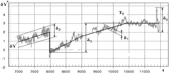
Fig. 1. Deviations plotted in % against the time of operation (hours)
A baseline functions ![]() is of a polynomial
type. A vector
is of a polynomial
type. A vector ![]() of functions’ arguments
comprises variables of ambient air pressure p*H, engine inlet temperature T*in, power turbine rotation speed nPT and fuel consumption Gf. Unknown polynomial coefficients were
estimated by the least square method with healthy engine data (reference set).
of functions’ arguments
comprises variables of ambient air pressure p*H, engine inlet temperature T*in, power turbine rotation speed nPT and fuel consumption Gf. Unknown polynomial coefficients were
estimated by the least square method with healthy engine data (reference set).
The baseline functions
were determined and the deviations were computed for all 6 gas path variables
available for monitoring in the analyzed power plant. Table 1 contains the list
of these variables with designations of the corresponding deviations and
normalization parameters ![]() .
.
Table 1. Monitored variables
No
Variable’s name
![]()
Designations
Relative
deviations
Normalized deviations
1
Compressor temperature T*C
0.00525
dTc
Z1
2
Exhaust gas temperature T*HPT
0.00453
dTt
Z2
3
Power turbine temperature T*LPT
0.00502
dTpt
Z3
4
Gas generator rotation speed nHP
0.00347
dNhp
Z4
5
Compressor pressure p*C
0.00869
dPc
Z5
6
Exhaust gas pressure p*HPT
0.00775
dPt
Z6
The EGT deviation plotted in Fig.1 is a result of great efforts to enhance deviation quality. For instance, some cases of sensors’ abnormal functioning were detected and the corresponding data were excluded from the analysis. The baseline functions were also optimized by choosing the best function type, arguments, and reference set to determine the function.
As a result of the optimization, the deviations have become good indices of engine deterioration. In Fig.1 we can clearly see two periods of EGT increase that is a result of compressor fouling, which is practically permanent and the most intensive deterioration mechanism of stationary gas turbines [5]. The periods are divided by a compressor washing in the time point t = 7970hours.
Figure 1 also helps us
to quantify quality of the deviations and specify deviation errors. The
deviation quality can be expressed by a ratio ![]() (signal-to-noise
ratio) of the maximum systematic change
(signal-to-noise
ratio) of the maximum systematic change ![]() to a spread
to a spread ![]() of deviation
fluctuations.
of deviation
fluctuations.
According to a frequency
and scatter, the fluctuations may be conditionally divided into three groups:
1) high frequency noise that is observed in every time point and has a scatter ![]() <0.3%, 2) slower fluctuations with the period of 30-300
hours and a scatter
<0.3%, 2) slower fluctuations with the period of 30-300
hours and a scatter ![]() <1.5%, 3) single spikes with a scatter
<1.5%, 3) single spikes with a scatter ![]() >1.5%. Since the spikes have the largest scatter, they can
nearly always be detected, identified and excluded from the analyzed data.
Generally, they are results of sensor malfunctions. To the contrary, the
fluctuations
>1.5%. Since the spikes have the largest scatter, they can
nearly always be detected, identified and excluded from the analyzed data.
Generally, they are results of sensor malfunctions. To the contrary, the
fluctuations ![]() resulted from
permanent measurement noise can not be removed. Being small, these fluctuations
do not however considerably affect diagnosis accuracy. A main obstacle in the
way to a correct diagnosis is related with the fluctuations
resulted from
permanent measurement noise can not be removed. Being small, these fluctuations
do not however considerably affect diagnosis accuracy. A main obstacle in the
way to a correct diagnosis is related with the fluctuations ![]() . On the one hand, their effect is sufficiently great; on the
other hand, it is often difficult to identify their origin. That is why these
fluctuations can be mistaken for the effects of engine deterioration resulting
in a misdiagnosis.
. On the one hand, their effect is sufficiently great; on the
other hand, it is often difficult to identify their origin. That is why these
fluctuations can be mistaken for the effects of engine deterioration resulting
in a misdiagnosis.
In addition to the graphical analysis conducted above, let us theoretically analyze possible causes and sources of the deviation errors that can take place in practice. This will help to understand their behavior and to take them into account with higher accuracy.
3. Theoretical analysis of possible errors in real deviations
This analysis takes into consideration our previous studies on deviation accuracy [4,6] and is performed below on the basis of expression (5) used to compute the deviations in real conditions. Although the expression looks to be simple, the analysis will not be so trivial.
3.1. Error types
For a monitored variable Y, expression (5) can be rewritten as
 . (7)
. (7)
This equation shows that
inaccuracy of the deviation is completely determined by errors in a term ![]() . It will be shown below that these errors can be divided
into four types. One type is connected with a measured value
. It will be shown below that these errors can be divided
into four types. One type is connected with a measured value ![]() and the other three types
are related to a function
and the other three types
are related to a function ![]() .
.
The measurement ![]() differs from a true
value Y by an error
differs from a true
value Y by an error ![]() called in this paper
as a Type I error. In its turn, the true value depends on a vector
called in this paper
as a Type I error. In its turn, the true value depends on a vector ![]() of real operating
conditions and on engine health conditions given by the vector
of real operating
conditions and on engine health conditions given by the vector ![]() . As a consequence, the value
. As a consequence, the value ![]() can be determined as
can be determined as
![]() . (8)
. (8)
The error ![]() is defined here as a
function because, in general, measurement errors may depend on the value Y and, consequently, on the variables
is defined here as a
function because, in general, measurement errors may depend on the value Y and, consequently, on the variables ![]() and
and ![]() .
.
One more obvious cause
of the deviation inaccuracy is related with measurement errors in operating
conditions presented in equation (7) by the vector ![]() . Given a vector of measurement errors
. Given a vector of measurement errors ![]() , which presents Type II errors, the measured operating
conditions are written as
, which presents Type II errors, the measured operating
conditions are written as
![]() . (9)
. (9)
The next error type
(Type III) is also related to engine operating conditions however it is not so
evident. The point is that not all real operating conditions denominated in the
present paper by a [(n+k)×1]-vector ![]() can be included as arguments of the baseline
function. Some variables of real operating conditions are not always measured
or recorded, for example, inlet air humidity, air bleeding and bypass valves’
positions, and engine box temperature. Let us unite all these additional
variables in a (k×1)-vector
can be included as arguments of the baseline
function. Some variables of real operating conditions are not always measured
or recorded, for example, inlet air humidity, air bleeding and bypass valves’
positions, and engine box temperature. Let us unite all these additional
variables in a (k×1)-vector ![]() . Since such variables exert influence upon a real engine and
its measured variable
. Since such variables exert influence upon a real engine and
its measured variable ![]() but are not taken into
consideration in the baseline function
but are not taken into
consideration in the baseline function ![]() , the corresponding deviation errors take place. A similar
negative effect can occur if sensor systematic error changes in time.
, the corresponding deviation errors take place. A similar
negative effect can occur if sensor systematic error changes in time.
Given that ![]() ,
the vector
,
the vector ![]() can
be given by
can
be given by ![]() and the equation (9)
is converted to a form
and the equation (9)
is converted to a form
![]() . (10)
. (10)
Apart from the described
errors related to the arguments of the function ![]() , the function has a proper error
, the function has a proper error ![]() (Type IV error). It
can result from such factors as a systematic error in measurements of the
variable Y, inadequate function type,
improper algorithm for estimating function’s coefficient, errors in the
reference set, limited volume of the set data, and influence of engine
deterioration on these data. Given
(Type IV error). It
can result from such factors as a systematic error in measurements of the
variable Y, inadequate function type,
improper algorithm for estimating function’s coefficient, errors in the
reference set, limited volume of the set data, and influence of engine
deterioration on these data. Given ![]() and a true function
and a true function ![]() , the function estimation
, the function estimation ![]() can be written as
can be written as
![]()
![]() . (11)
. (11)
3.2. Deviation formula
Let us now substitute
equations (8), (10), and (11) into expression (7). As a result, the deviation ![]() is written as
is written as
 . (12)
A dependency ![]() in this expression can
be simplified because of the following reasons: a)
in this expression can
be simplified because of the following reasons: a) ![]() , b)
, b) ![]() , c) The influence of
, c) The influence of ![]() and
and ![]() on Y and, consequently, on
on Y and, consequently, on ![]() is significantly
smaller then the influence of
is significantly
smaller then the influence of ![]() . Taking into account the considerations made, we arrive to a
final expression for the deviation
. Taking into account the considerations made, we arrive to a
final expression for the deviation
 . (13)
This expression includes
four error types introduced above, namely ![]() ,
,![]() ,
, ![]() , and
, and ![]() . Let us now analyze how each error can influence on
inaccuracy of the deviation
. Let us now analyze how each error can influence on
inaccuracy of the deviation ![]() .
.
3.3. Influence of different error types
The influence of
different error sources on the deviations are analyzed in the sequel under the
following assumptions commonly applied in gas turbine diagnostics. First, the
same sensors were employed to measure currently analyzed values ![]() and
and ![]() as well as the
reference set data. Second, gross errors (e.g. spikes) have been filtered out.
Third, a systematic error and amplitude of random errors in
as well as the
reference set data. Second, gross errors (e.g. spikes) have been filtered out.
Third, a systematic error and amplitude of random errors in ![]() and
and ![]() do not depend on
engine operating time.
do not depend on
engine operating time.
Type I error. Since the
sensor performance is invariable, every systematic change of the error ![]() will be accompanied by
the same change in
will be accompanied by
the same change in ![]() . As a consequence, accuracy of the deviation
. As a consequence, accuracy of the deviation ![]() will not be affected
by the systematic component of
will not be affected
by the systematic component of ![]() . As to the random component, it is usually given by the
Gaussian distribution. It is also believed that random errors of different
variables Y are independent and are
described by the multidimensional Gaussian distribution. That is why, the
corresponding errors in the deviations
. As to the random component, it is usually given by the
Gaussian distribution. It is also believed that random errors of different
variables Y are independent and are
described by the multidimensional Gaussian distribution. That is why, the
corresponding errors in the deviations ![]() of these variables can
also be described by this distribution.
of these variables can
also be described by this distribution.
Type II errors. Errors ![]() can be analyzed in the
same way as the Type I errors, separately for systematic and random components.
Obviously, the objective of a function determination method (e.g. least square
method) is to minimize the distance between the reference set data and function
outputs. That is why, a baseline function will correctly describe reference
data regardless of the systematic errors in function arguments (systematic
component of the error
can be analyzed in the
same way as the Type I errors, separately for systematic and random components.
Obviously, the objective of a function determination method (e.g. least square
method) is to minimize the distance between the reference set data and function
outputs. That is why, a baseline function will correctly describe reference
data regardless of the systematic errors in function arguments (systematic
component of the error ![]() ). Since the systematic error component is the same in the reference
set and in a currently measured argument vector
). Since the systematic error component is the same in the reference
set and in a currently measured argument vector ![]() , a function output
, a function output ![]() will be adequate to a
measured value
will be adequate to a
measured value ![]() . In this way, the system component of the errors
. In this way, the system component of the errors ![]() cannot influence a lot
the deviation
cannot influence a lot
the deviation ![]() .
.
As to the random
component, it can be described by the multidimensional Gaussian distribution,
as in the case of the monitored variables Y.
Because every change of the arguments ![]() has an influence on baseline
values of all monitored variables, their baseline values
has an influence on baseline
values of all monitored variables, their baseline values ![]() and, consequently,
deviations
and, consequently,
deviations ![]() may have correlation.
Thus, independent random errors of measured operating conditions can induce
correlated deviation errors that cannot be described by the multidimensional
Gaussian distribution.
may have correlation.
Thus, independent random errors of measured operating conditions can induce
correlated deviation errors that cannot be described by the multidimensional
Gaussian distribution.
It is very likely that
the noise with a scatter ![]() observed in Fig.1
results from a random component of the errors of Type I and Type II.
observed in Fig.1
results from a random component of the errors of Type I and Type II.
Type III error. Presence
of such an error has been confirmed after analyzing all other error types. This
error occurs because the additional operating conditions ![]() do not change baseline
function but exert influence on a real engine and, accordingly, on all
variables Y. For this reason, any
change of
do not change baseline
function but exert influence on a real engine and, accordingly, on all
variables Y. For this reason, any
change of ![]() can induce synchronous
errors of the deviations
can induce synchronous
errors of the deviations ![]() of all monitored variables.
It is very likely that most fluctuations with the scatter
of all monitored variables.
It is very likely that most fluctuations with the scatter ![]() (see Fig.1) origin
from the Type III errors.
(see Fig.1) origin
from the Type III errors.
Type IV error. The
issue of the baseline function non-adequacy {error ![]() } is a particular case of a well studied mathematical problem
of the function estimation with empirical data [7]. This error varies in time along
with changes in the operating conditions
} is a particular case of a well studied mathematical problem
of the function estimation with empirical data [7]. This error varies in time along
with changes in the operating conditions ![]() producing
perturbations in the deviation variable
producing
perturbations in the deviation variable ![]() . These perturbation can be both independent and correlated
depending on particular causes of the error
. These perturbation can be both independent and correlated
depending on particular causes of the error ![]() . Although the baseline function adequacy is a challenge, the
error can be reduced to an acceptable level by applying a proper function type and
using a representative reference set.
. Although the baseline function adequacy is a challenge, the
error can be reduced to an acceptable level by applying a proper function type and
using a representative reference set.
A deviation plot in Fig.1 is a result of multiple attempts to enhance deviation quality. The achieved deviation accuracy is not inferior to the level known from the literature and is sufficient for reliable monitoring of the power plant under analysis. Thus, we can conclude that Fig. 1 gives an example of deviation errors expected in a real situation. Therefore, to obtain realistic results of gas turbine diagnosis, simulated noise should be as close as possible to such real errors. This is verified below by comparing different schemes to represent deviation errors.
4. Noise representation schemes
4.1. Real error extraction
To extract an error component from the
deviations based on real data, a model ![]() of an degraded power
plant has been firstly determined as shown in [4,6]. In addition to the
operating conditions
of an degraded power
plant has been firstly determined as shown in [4,6]. In addition to the
operating conditions ![]() , the monitored variable Y
depends in this model on engine operation time after the last washing
, the monitored variable Y
depends in this model on engine operation time after the last washing ![]() . Model’s coefficient were computed by the least square
method with the reference set that includes the first 2500 operating points
presented in Fig.1. A baseline model
. Model’s coefficient were computed by the least square
method with the reference set that includes the first 2500 operating points
presented in Fig.1. A baseline model ![]() was then simply
determined by putting
was then simply
determined by putting ![]() equal to zero.
equal to zero.
With the described model and equation (6), a
relative deviation error ![]() is
written as
is
written as
 (14)
(14)
The errors ![]() of
all monitored variables were computed for the 2500 points of the reference set
as well as for 1400 subsequent operating points of an additional sample called
a testing set. Plots of Fig. 2 illustrate the relative errors
of
all monitored variables were computed for the 2500 points of the reference set
as well as for 1400 subsequent operating points of an additional sample called
a testing set. Plots of Fig. 2 illustrate the relative errors ![]() of the reference set. With these errors the normalization
parameters were estimated for each monitored variable according to an
expression
of the reference set. With these errors the normalization
parameters were estimated for each monitored variable according to an
expression ![]() , where
, where ![]() denotes a standard
deviation of the variable
denotes a standard
deviation of the variable ![]() . The resulting
values
. The resulting
values ![]() are given in Table 1.
are given in Table 1.
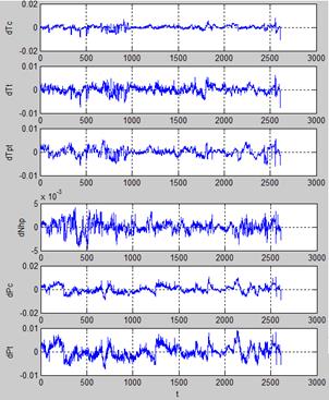
Fig.2. Relative errors computed for the reference set
Three error representation
schemes are realized and examined below. Since a diagnostic space is formed by
the normalized deviations ![]() [see equation (4)],
the corresponding normalized errors
[see equation (4)],
the corresponding normalized errors ![]() are considered in all
schemes. These errors, both real and simulated, were computed with the same
normalization parameters of Table 1.
are considered in all
schemes. These errors, both real and simulated, were computed with the same
normalization parameters of Table 1.
4.2. Scheme A: sensor error simulation
This scheme is the most widely applied in gas turbine fault recognition algorithms. The errors of each measured quantity, monitored variable Y or operating condition U, are usually given by the normal distribution. To simulate these errors (errors of Type I and Type II), we used the standard deviations σ of sensor uncertainties given in Table 2. These parameters were chosen in our previous work [8] on the basis of multiple literature sources. The influence of errors of the operating conditions on the monitored variables was estimated with the thermodynamic model described in section 1.
Table 2. Measurements uncertainties (σ,%)
|
p*H |
T*in |
nPT |
Gf |
T*C |
T*HPT |
T*LPT |
nHP |
p*C |
p*HPT |
|
0,03 |
0,2 |
0,1 |
0,5 |
0,2 |
0,25 |
0,2 |
0,05 |
0,2 |
0,3 |
Figures 3 and 4a illustrate the considered schemes. It is clearly seen in Fig.4a that the presented deviation errors (deviations of exhaust gas temperature and power turbine temperature) have correlation. It is also visible that the error span considerably exceeds the interval (-1.0,1.0), i.e. the deviation errors induced by the simulated sensor noise are more dispersed than the real errors computed for the reference set data.
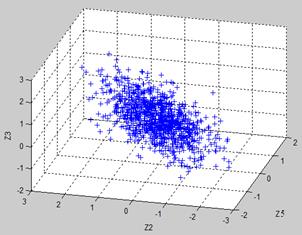
Fig.3. 3D plot of the normalized deviation errors according to Scheme A (deviation designations Z5, Z2 and Z3 correspond to Table 1)
|
a) Scheme A: sensor error simulation |
b) Scheme B: deviation error simulation |
|
c) Scheme C: real deviation errors (reference set) |
d) Scheme C: real deviation errors (testing set) |
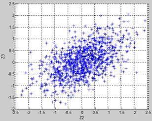
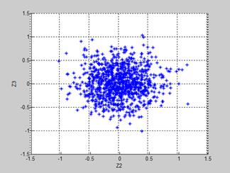
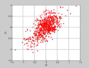
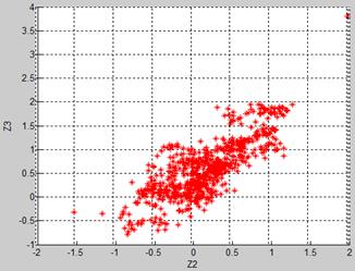
Fig. 4. 2D plots for different schemes of deviation error representation
(deviation designations Z2 and Z3 correspond to Table 1)
4.3. Scheme B: direct simulation of the deviation errors
This scheme was applied to simulate fault classes in our previous works (see, for instance, [9]). The deviation errors are given by the multidimensional normal distribution. The same standard deviations that were obtained for real noise are chosen. This allows exact adjustment of simulated errors to real ones.
This scheme is illustrated by Fig.4b. As it was expected, practically all simulated normalized errors are distributed inside the intervals (-1.0,1.0) and no correlation is observed. The latter can be considered as a disadvantage because the correlation produced by Type II errors and expected in real deviations is absent.
4.4. Scheme C: errors of real deviations
This scheme is proposed and it means the integration of the normalized deviation errors computed with real data in the description of simulated faults. The scheme was realized separately for the cases of the reference and testing sets. The corresponding deviation errors are illustrated by Fig.4c and Fig.4d. As expected, the errors computed for the reference set (Fig.4c) are mostly localized inside the intervals (-1.0,1.0) while the errors of the training set have significantly wider dispersion. Both figures show visible error correlation between the presented deviations. It also can be seen that the distribution of real errors, especially for the case of the testing set, is les regular than the simulated error distributions presented in Fig4a and Fig 4b.
In this way, we can conclude that simulated deviation errors can differ a lot from real errors. Consequently, this can affect the accuracy of estimated indicators of gas turbine diagnosis reliability.
4.5. Influence of different noise representation schemes on diagnosis reliability: first results
With three described above schemes of noise representation, three corresponding fault classifications have been formed for the analyzed power plant. Namely, three variations of the learning and validation sets were created. Each classification includes 9 classes and each class is simulated by the gradual change of the corresponding fault parameter in the thermodynamic model. Four such classes are shown in Fig.5 in the space of three normalized deviations. The deviation errors correspond to scheme A.
Multilayer perceptron, the
most widely used network, was chosen to recognize the faults. It was trained
consequently with each variation of learning data. The probabilities of true diagnosis ![]() and
and ![]() (see section 1) have
been computed by applying this network to the
corresponding variation of validation data.
(see section 1) have
been computed by applying this network to the
corresponding variation of validation data.
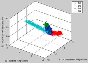
Fig.5. 3D plot of fault classes in the space of normalized deviations (Scheme A)
Preliminary calculations have shown that the distinguishability of fault classes can change by up to 6% when real errors are replaced by simulated errors. Thus, the diagnostic performance estimated with simulated noise can be inaccurate.
The case was also investigated of learning data
with reference set errors (see Fig4c) and validation data with testing set
errors (Fig4d). Since real errors obtained from the testing set are more
dispersed, we expected some degradation of the power plant diagnosability. The
degradation was found drastic: from ![]() = 90% - 94% in the
previous cases to
= 90% - 94% in the
previous cases to ![]() = 59%. It happened
because the model of degraded engine determined on the reference set has lost
its accuracy on the testing set. Such a problem seems to be very probable in
real diagnosis and we should be careful to avoid or mitigate it.
= 59%. It happened
because the model of degraded engine determined on the reference set has lost
its accuracy on the testing set. Such a problem seems to be very probable in
real diagnosis and we should be careful to avoid or mitigate it.
Conclusions
Thus, possible errors in deviations of gas turbine monitored variables have been analyzed in this paper. The problem of deviation accuracy is important because no monitored variables themselves but their deviations are input parameters in diagnostic algorithms.
A power plant for natural gas pumping has been chosen as a test case. It was presented in the present study by its nonlinear thermodynamic model and the data recorded under field conditions.
Possible deviation errors have been investigated theoretically and graphically. All error sources were thoroughly examined and classified into four types. We succeeded in finding a single mathematical expression to relate the deviation with its typical errors.
Three alternative schemes, two existing and one new, of deviation error representation in diagnostic algorithms have been realized. They were compared with the use of graphical means and probabilities of correct diagnosis. Preliminary results show that the existing schemes of error simulation do not always ensure the necessary accuracy of estimated engine diagnosability. The new scheme enhances the accuracy by including the noise component obtained from real data into the description of fault classes.
Although the proposed scheme is more realistic, it cannot automatically replace existing noise simulation modes. This scheme is more complex for realization. Additionally, it needs both the thermodynamic model and extensive real data, two things rarely available together. In this way, the proposed scheme of deviation error representation can rather be recommended for a final precise estimation of gas turbine diagnosability.
This paper can only be considered as a preliminary study. The investigations will be continued to better investigate this new scheme and to draw the final conclusion on its applicability in gas turbine diagnostics.
Acknowledgments
The work has been carried out with the support of the National Polytechnic Institute of Mexico (research project 20113092).
References
1. Roemer M.J. An Overview of Selected Prognostic Technologies with Application to Engine Health Management / M.J. Roemer, C.S. Byingto, G. Kacprzynski, G. Vachtsevanos. − Proc. ASME Turbo Expo 2006, Barcelona, Spain, 2006. − 9 p.
2. Miro Zarate L.A. Mejoramiento de la simulacion de fallas de turbinas de gas / L.A. Miro Zarate, I. Loboda, E. Torres Garcia. − Memorias del 12o Congreso Nacional de Ingenieria Electromecanica y de Sistemas, Mexico, 2010. − P. 576-581.
3. Duda R.O. Pattern Classification / R.O. Duda, P.E. Hart, D.G. Stork. − Wiley-Interscience, New York, 2001.
4. Loboda I. Deviation problem in gas turbine health monitoring / I. Loboda, S. Yepifanov, Y. Feldshteyn. − Proc. IASTED International Conference on Power and Energy Systems, Clearwater Beach, Florida, USA, 2004. − P. 335-340.
5. Mejer-Homji C.B. Gas turbine performance deterioration / C.B. Mejer-Homji, M.A. Chaker, H. M. Motiwala. − Proc. Thirtieth Turbomachinery Symposium, Texas, USA, 2001. − P. 139-175.
6. Loboda I. Diagnostic analysis of maintenance data of a gas turbine for driving an electric generator / I. Loboda, S. Yepifanov, Y. Feldshteyn // International Journal of Turbo & Jet Engines. − 2009. − Vol. 26, Is. 4. − P. 235-251.
7. Vapnik V. Estimation of Dependencies Based on Empirical Data / V. Vapnik. − Springer Verlag, New York, 1982.
8. Maravilla Herrera C. A comparative analysis of turbine rotor inlet temperature models / C. Maravilla Herrera, S. Yepifanov, I. Loboda. − Proc. ASME Conference Turbo Expo 2011, Vancouver, Canada, 2011. − 11 p.
9. Loboda I. A generalized fault classification for gas turbine diagnostics on steady states and transients / I. Loboda, S. Yepifanov, Y. Feldshteyn // Journal of Engineering for Gas Turbines and Power. − 2007. − Vol. 129, Is. 4. − P. 977-985.