Loboda Igor

There are various types of gas turbine deterioration and faults such as fouling, tip rubs, seal wear, erosion, and foreign object damage. Since such real defects occur rarely during maintenance, the thermodynamic model is a unique technique to create necessary class descriptions. To take into account the component performance changes induced by real gradual deterioration mechanisms and abrupt faults, the fault parameters that shift a little the components’ maps as shown in Fig.1.

Mathematically, the model is a system of nonlinear algebraic equations reflecting mass, heat, and energy balance for all components operating under stationary conditions.

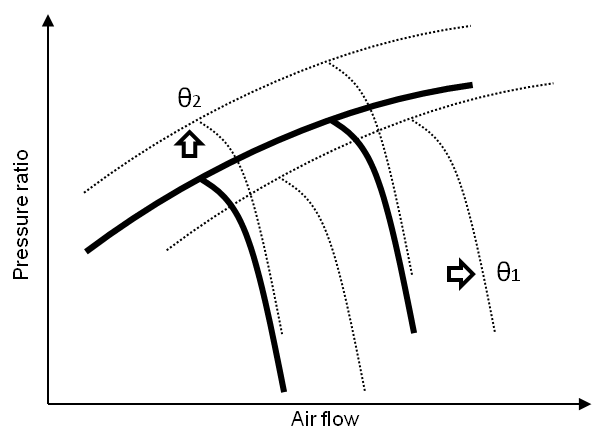
Fig. 1. Compressor map shifting by the fault parameters

The thermodynamic model for steady states has wide applications in gas turbine diagnostics. First, as shown before and in more detail in [5], this model is used to describe particular faults or complete fault classification. Second, the thermodynamic model is an integral part of numerous diagnostic algorithms based on system identification such as described in [6]. Third, this nonlinear model allows computing simpler models, like a linear model used in [7] and in the present paper to create flexible fault classifications.

2. Linear static model

The linear static model presents linearization of nonlinear dependency between gas path variables and fault parameters determined for a fixed operating condition . The model is given by a vectorial expression:

It connects a vector of small relative changes of the fault parameters with a vector of the corresponding relative deviations of the monitored variables by a matrix of influence coefficients (influence matrix).

Since linearization errors are not too great, about some per cent, the linear model can be successfully applied for fault simulation at any fixed operating point. However, when it is used for estimating fault parameters by system identification methods like in study [6,8], estimation errors can be significant. Given the simplicity of the linear model and its utility for analytical analysis of complex diagnostic issues, this model will remain important in gas turbine diagnostics.

2. Methodology for gas turbine diagnosis

2.1 Deviations

By direct analysis of the variables themselves it is difficult to discriminate performance degradation effects from great changes due to different operating modes. To draw useful diagnostic information from raw recorded data, a total gas turbine diagnostic process usually includes a preliminary procedure of computing deviations. The deviations are defined as differences between measured and engine baseline values. As the baseline depends on an engine operating condition, it can be written as function ( usually called a baseline function. With this model the deviations for each monitored variables is computed in a relative form:

where denotes a measured value.

2.2 Diagnostic space

As mentioned before, models are used in gas turbine diagnostics to describe engine performance degradation and faults and the deviations are employed to reveal the degradation influence. These deviations are written in relative form and normalized so as to facilitate simulating faults and their subsequent recognition. At a steady state, the deviation is defined for i-th measured variable as:

where is the amplitude of possible random fluctuations in the original deviation . To take into account possible measurement errors, the vector of random variables distributed within the interval (-1,1) is added. A resultant vector

corresponds to the deviations that are calculated in practice for actual measurements.

2.3 Principles for developing classification

Engine faults vary considerably. Hence, for the purposes of engine diagnostics this variety has to be broken down into a limited number of classes. In the pattern recognition theory, it is often supposed that an object state can belong only to one of present classes

Consequently

We accept this hypothesis for a gas turbine fault classification.

Fault classifications can contain two different types of fault classes: singular or multiple classes. The first type works with only one fault parameter while the second one is formed by independent changes of two or more fault parameters in order to represent more complex faults in gas turbines.

For each class, singular or multiple, numerous patterns are generated according to expression (4) setting the necessary quantities and by the uniform and Gaussian distributions accordingly. A typical number of patterns per class is 1000. A totality of all classification’s patterns is employed to train the used neural network and is therefore called a learning set.

2.4 Recognition decision making

A nomenclature of possible diagnosis made by a recognition technique (neural network within the present paper) corresponds to the accepted classification (6). To make a diagnosis a criterion specific for each technique is introduced as a measure of membership of a current pattern in class . To determine the functions , a learning set is used. After calculating all values , a decision rule

is applied.

2.5 Recognition accuracy

To verify a recognition technique determined with the help of the learning set, one more set is required. The necessary set , called a validation set, is created in the same way as the set . The only difference is that other series of random numbers is generated to simulate fault severity and errors in the deviations.

Every pattern in the validation set belongs to a known class. Comparing this class with the diagnosis , we can compute probabilities and compose a confusion matrix (Table 1). Its diagonal elements form a vector of true diagnosis probabilities that are indices of classes’ distinguishability. Mean number of these elements – scalar – characterizes total engine diagnosability. No diagonal elements are wrong diagnosis probabilities. They help to identify the causes of bad class distinguishability. For 1000 patterns per class, the computational precision of the mean probability is approximately ±0.01. In order to enhance the precision, each calculation of is repeated in the present study 100 times, each time with new series of random numbers. The 100 corresponding random values of are averaged, resulting in a probability P_av with higher precision of ±0.001.

Table 1

Confusion matrix

3. Pattern recognition techniques

Three different artificial neural networks described below have been chosen in the present study for gas turbine fault recognition.

3.1 Multi-Layer Perceptron (MLP)

The MLP is a feedforward artificial neural network model that maps sets of input data onto a set of appropriate outputs. It consists of multiple layers of nodes in a directed graph, with each layer fully connected to the next one. Except for the input nodes, each node is a neuron with a nonlinear activation function (Fig. 2). When the perceptron is applied to a classification problem, each output k gives a closeness measure between the analyzed input pattern and a class .

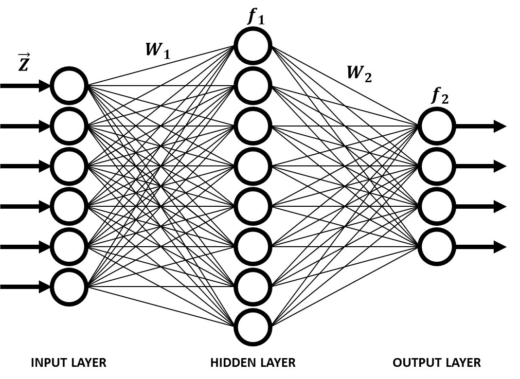
Fig. 2. Typical MLP structure

During the learning, unknown weight coefficients and biases are determined by a back-propagation algorithm, in which a network output error is propagated backwards to correct these unknown quantities. They are corrected in the direction that reduces the error unless a global error minimum is reached. The back-propagation algorithm needs differentiable transfer functions and they usually are of a sigmoid or linear type. MLP is a modification of the standard linear perceptron and can distinguish data that are not linearly separable

3.2 Radial Basis Network (RBN)

A RBN is an artificial neural network that uses radial basis functions as activation functions. The output of the network is a linear combination of radial basis functions of the inputs and neuron parameters. A radial basis neuron operates as follows. Neuron's weight coefficients form a weight vector that is one of learning patterns. First, a distance between the weight vector and an input vector is computed. This distance is then divided by a bias b resulting in an input n to a radial basis transfer function (RBF). The RBF finally computes a neuron’s output according to an expression . When the distance is 0, this function has a maximum value . The function decreases when the distance increases. The bias b allows changing an action area (window) of the neuron and is called spread. The output layer of the RBN works similarly to a usual perceptron output layer with a linear transfer function.

3.3 Probabilistic Neural Network

A probabilistic network, specific type of radial basis networks, is specially intended for classification problems. It consists of three layers. The hidden layer is formed and operates just like the same layer of the RBN algorithm. It is built from learning patterns united in a matrix . Each learning pattern specifies a center of the RBN of one hidden neuron. A Euclidean distance between the function center and the input pattern is firstly computed. The distance divided by the spread b is a hidden neuron input. A radial basis function then calculates a neuron output . The closer the input vector is situated to the neuron center, the greater the neuron output will be. Thus, elements of a vector indicate how close the input pattern is to the learning patterns.

The output or classification layer differs from the RBN output layer. Each classification neuron corresponds to one of the analyzed classes. An input of the classification neuron, which is interpreted as a probability of this class, is computed as a sum of the signals related with the learning patterns of the same class. In other words, each hidden neuron is connected with only one classification neuron and connection weights are equal to one. To realize such a connection, a matrix is composed in a particular way from zero and one elements and a product is computed. It is an input vector for the classification layer and consists of probabilities of all considered classes. Finally, the classification layer transfer function produces a 1 corresponding to the largest probability, and 0's for the other network outputs. Thus, the PNN classifies the input vector into a specific class on the basis of a probability measure.

4. Calculation conditions

The approach and three neural networks described above were applied for diagnosing a turboshaft stationary power plant with a free turbine intended for driving a centrifugal compressor in natural gas pipelines. Five components of the engine are diagnosed: inlet device, axial compressor, combustion chamber, compressor turbine and power turbine. An engine operating point is given by a constant compressor rotational speed 10700 rpm and standard atmospheric conditions. The six gas path variables of Table 2 corresponding to an engine standard measurement system are available for monitoring. To simulate gas path and measurement system faults, the eighteen fault parameters from Table 3 are involved.

Table 2

Monitored variables

* component pressures and temperatures correspond to a component discharge section

Table 3

Fault parameters

On the basis of the fault parameters specified in Table 3, the next section introduces various fault classification variations.

5. Fault classification variations

With the intention of studying the influence of the fault classification structure on final diagnostic accuracy, twelve fault variations are introduced. These variations contain different class quantities, fault parameters, fault development directions (positive or negative) and engine components. These variations are specified in Table 4 and additionally briefly described below.

• Variation 1: It has nine singular classes formed by gas path parameters whose changes are negative.

• Variation 2: It is formed by four multiple classes with two gas path parameters per class and grouped by an engine component: compressor, turbine, power turbine and combustion chamber (Fig. 3).

• Variation 3: The combination of variation 1 and three singular classes with positive direction of a fault parameter (turbine and power turbine air flow parameters and combustion chamber pressure ratio) to simulate burns in hot parts.

• Variation 4: The combination of variation 2 + three multiple classes formed by turbine and power turbine air flow parameters, combustion chamber pressure ratio and their respective efficiencies (negative direction).

• Variation 5: It contains six singular classes of sensor faults in 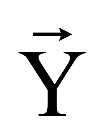. Each of them has positive and negative directions of fault.

• Variation 6: The combination of variations 3 and 5 resulting in eighteen singular classes to simulate gas path faults and sensor errors.

• Variation 7: Formed by seven multiple classes of variation 4 and six singular classes (sensor faults) with double limits.

• Variation 8: It has the six sensor faults in and three singular classes of sensor faults in .

• Variation 9: Formed by three multiple classes (turbine and power turbine air flow parameters, combustion chamber pressure ratio and their respective efficiencies) and one multiple class of faults in compressor.

• Variation 10: It contains nine singular classes: three singular classes with double direction of fault (turbine and power turbine air flow parameters and combustion chamber pressure ratio), four efficiencies for all components, one for the compressor air flow and another one for the inlet pressure loses factor.

• Variation 11: In this variation, each class is created by four fault parameters. It is formed by the combination of air flow parameters (with the exception of the combustion chamber pressure ratio) and efficiencies. The first three classes are formed by combining the turbine, the power turbine and the combustion chamber with the compressor, the fourth and the fifth - by combining the power turbine and the combustion chamber with the turbine. The last class is formed as the combination of the power turbine and the combustion chamber (Fig. 4).

• Variation 12: It is practically the same as variation 11, but, in this case all the classes have negative directions to simulate gas path faults.

For each classification variation, fault diagnosis was performed by with three neural networks: Multi-Layer Perceptron, Radial Basis Network and Probabilistic Neural Network and the probability P_av and execution time were determined for each network. Table 5 shows all the results. All the computation was performed in a Dell Inspiron One Desktop: Intel Pentium G2020T processor, 2.5 GHz, and 4 GB of RAM.

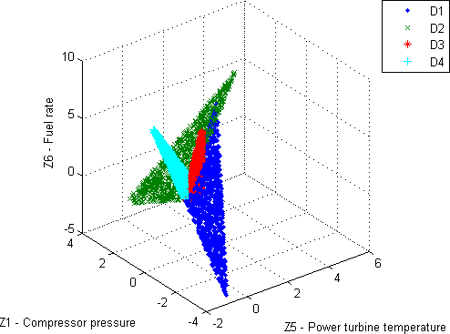
Fig. 3. Classification variation 2: four multiple classes with two fault parameters

Analyzing the probabilities, one can state that the differences between the networks within the same classification variation are not great (excepting variation 6),

about 0.015 (1.5%), while the difference between the variations can reach the value 0.10. Thus, these results reaffirm once more the conclusion drawn in [9] that many recognition techniques may yield the same gas turbine diagnosis accuracy.

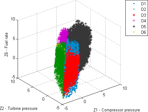
Fig. 4. Classification variation 11: six multiple classes with four fault parameters

The execution time includes 100 cycles of calculation of the mean probability . Each cycle consists of a learning stage with thousands diagnosis cycles of a validation stage at which the probability is computed. In Table 5, we can see that this total time is by far smaller for the PNN for all classifications. This is explained by the fact that this network does not need a learning stage. Thus, the PNN seems to be the simplest network to tailor for gas turbine diagnosis.

Table 4

Variations of classification and their fault class formation

6. Boundaries for multiple fault classes

When multiple faults are simulated by summing the influence of each fault parameter, there is the risk that the simulated fault exceeds a severity limit of real faults. In Fig.3, a multiple class D₁ created by two fault parameters is illustrated. The point “0” corresponds here to an engine normal state. Each of the vectors OL₁ and OL₂ results from the change of one fault parameter. Points L₁ and L₂ and vector lengths l₁ and l₂ correspond to an engine health limit. An area of deviation vectors without errors presents a parallelogram and area corresponds to deviation vectors with errors. It can be seen that vectors in the upper right corner of the parallelogram can be longer than base vectors OL₁ and OL₂ produced by a maximal change of the corresponding fault parameters. In other words, simulated faults can have higher severity than real ones.

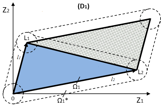
Fig. 5. Straight line boundary

To make the simulated faults more realistic, we previously used a linear boundary L₁L₂ that restricts fault pattern vectors inside the triangle OL₁L₂. However, this boundary becomes too restrictive when the angle L₁OL₂ increases.

An ideal boundary seems to us like a smooth curve formed by a vector that turns from OL₁ to OL₂ and gradually changes its length from l₁ to l₂ proportionally to the turning angle. It is proposed to express this length by:

where is the angle between a current vector and the first base vector and is the angle between the two base vectors. As can be seen, the boundary determined by (9) corresponds to the Archimedean spiral. Figure 6 illustrates action of the proposed boundary: the deviation vectors that are inside the curve are only accepted.

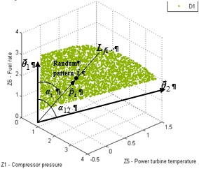
Fig. 6. Archimedeaspiral boundary

(Two fault parameters)

The described boundary rule can be easily extended on the case of three fault parameters illustrated by Fig.7. The boundary vector of the length l determined in the plane of the first and second fault parameters (orange area) is considered as a base vector. The second base vector OL₃ is produced by the third fault parameters. The boundary is determined in the plane of these two base vectors (green area). For the case of four and more fault parameters, we only need to repeat the above procedure.

To better understand the importance of the new boundary, three boundary options have been examined: no boundary (parallelogram area ), straight line (triangle area ), and Archimedean spiral. The boundaries were applied for multiple faults of classification variations 2 and 12. For each option and each variation, the three selected neural networks were used by turn for computing average true diagnosis probabilities P_av. Table 6 contains all the results, which help to draw the following conclusions. First, the new boundary results in a visible change of the probability P_av (up to 0.04). This change can be greater for particular fault classes. Second, for all cases the “Archimedean spiral” probability occupies an intermediate position between “No boundary” probability and “Straight line” probability. This is naturally explained by the fact that the Archimedean spiral curve is situated between the straight line and the parallelogram sides. Third, for the new boundary, the difference between the recognition techniques (three networks) remains small: 0.0045 for classification variation 2 and 0.0133 for variation 12.

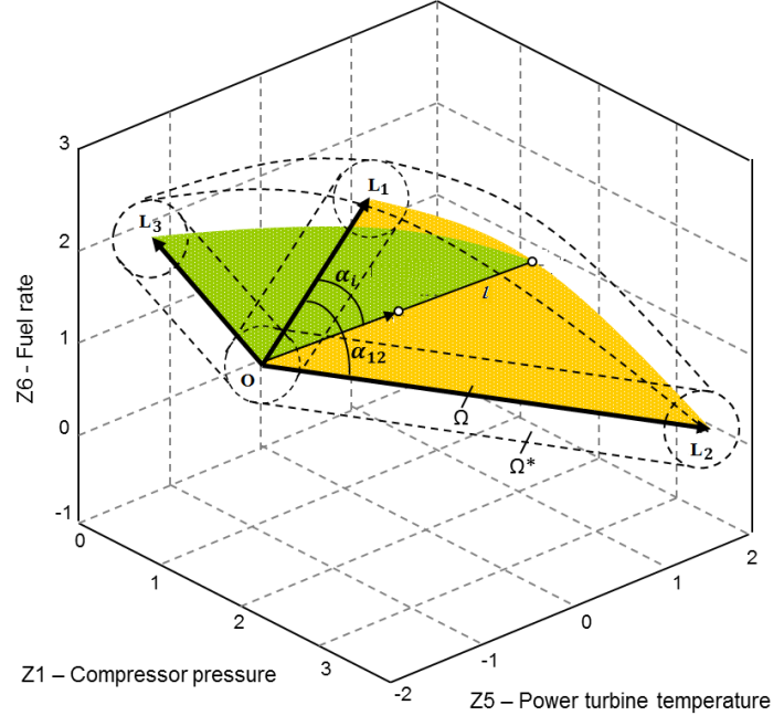
Fig. 7. Archimedean spiral boundary

(Three fault parameters).

Table 5

Average true diagnosis probabilities P_av for different classification variations.

Table 6

Average true diagnosis probabilities P_av for different fault severity boundaries

Conclusions

In investigations and practice of gas turbine diagnosis, fault classifications vary considerably. That is why, the present paper proposes a flexible fault classification that allows creating any necessary totality of fault classes of different types. Twelve classification variations were introduced and investigated in the paper. For each variation, an average probability of correct fault diagnosis was determined using by turn on of three neural networks as a fault recognition technique. Additionally, a new boundary that restricts fault severity was proposed and examined. The following conclusions have been drawn as a result of the investigations.

- The procedure of flexible classification has proven to create any necessary totality of fault classes of different type y complexity. Formation of a new classification variation and change from one variation to another is simple and does not need reprogramming the software.

- For all classification variation examined, three networks provide practically equal average probability of correct diagnosis. This confirms the conclusion made in previous studies that many recognition techniques can have the same diagnostic accuracy.

- Among the three networks, the probabilistic neural network seems to be simplest gas turbine fault recognition technique.

- The new boundary (Archimedean spiral) proposed for restricting the severity of simulated faults makes the simulation more realistic and allows to determine more precisely the level of diagnostic accuracy.

Acknowledgments

The work has been carried out with the support of the National Polytechnic Institute of Mexico (research project 20144199) and the National Council of Science and Technology (CONACYT).

References

1. Romessis, C. Bayesian Network Approach for Gas Path Fault Diagnosis [Text] / C. Romessis, K. Mathioudakis // ASME Journal of Engineering for Gas Turbines and Power. − 2006. − Vol. 128, Issue 1. − P. 64-72.

2. Loboda, I. Gas Turbine Fault Recognition Trustworthiness [Text] / I. Loboda, S. Yepifanov // Cientifica, Revista del Instituto Politecnico Nacional de Mexico. − 2006. − Vol. 10, Is. 2. − P. 65-74.

3. Butler, S. An Assessment Methodology for Data-Driven and Model Based Techniques for Engine Health Monitoring [Text] / S.W. Butler, K.R. Pattipati, A.J. Volponi // Proc. IGTI/ASME Turbo Expo 2006, Barcelona, Spain, May 8-11, 2006. − 9 p.

4. García Díaz, J. Diagnóstico de Turbinas de Gas con el Criterio de la Densidad de Probabilidad [Text] / J. García Díaz, I. Loboda, J.L. Pérez Ruiz // Proceedings of the VII International Congress of Electromechanical and Systems Engineering, Mexico City, Mexico, Oct 27-31, 2014. -7p.

5. Loboda, I. A Generalized Fault Classification for Gas Turbine Diagnostics on Steady States and Transients [Text] / I. Loboda, S. Yepifanov, Ya. Feldshteyn // Journal of Engineering for Gas Turbines and Power.-2007.- Vol.129, No.4.- P. 977-985.

6. Pinelli, M. Gas Turbine Field Performance Determination: Sources of Uncertainties [Text] / M. Pinelli, P.R. Spina // Journal of Engineering for Gas Turbines and Power.-2002.- Vol.124, No.1.- P. 155-160.

7. Pérez Ruiz, J.L. Clasificación Flexible de Fallas para el Diagnóstico Paramétrico de Turbinas de Gas [Text] / J.L. Pérez Ruiz, I. Loboda, I. González Castillo // Proceedings of the VII International Congress of Electromechanical and Systems Engineering, Mexico City, Mexico, Oct 27-31, 2014. -8p.

8. Kamboukos, Ph. Comparison of Linear and Nonlinear Gas Turbine Performance Diagnostics [Text] / Ph. Kamboukos, K. Mathioudakis // Journal of Engineering for Gas Turbines and Power.-2005.- Vol.127, No.1.- P. 49-56.

9. Loboda, I. Gas turbine fault recognition using probability density estimation [Text] / I. Loboda // Proceedings of the ASME Turbo Expo 2014 International Technical Congress, Dusseldorf, Germany, June 16-20, - 2014. - 13p., ASME Paper No. GT2014-27265.