Loboda Igor

Probability density estimation techniques for gas turbine diagnosis.

1 Introduction

It is a standard worldwide practice to apply health monitoring systems to detect, identify, and predict gas turbine faults. The diagnostic algorithms using gas path models and measured variables constitute an important integral part of these systems. Many of the algorithms apply pattern classification techniques, mostly different artificial neural networks [1-3].

Effectiveness of the monitoring system strongly depends on accuracy of its diagnostic decisions. That is why all system algorithms including the used classification technique should be optimized.

Among the neural networks applied to diagnose gas turbines, a multilayer perceptron (MLP) is the most widely used [3]. In our previous studies [4,5], diagnostic accuracy of the perceptron and some other classification techniques has been examined. It was found that on average four techniques including the MLP provide equally good results. Thus, to choose the best technique any additional criterion is required. The ability to accompany every diagnostic decision by a confidence measure is an important property of some classification techniques that can be accepted as such a criterion.

The present paper deals with two classification methods, Parzen Windows (PW) and K-Nearest Neighbors (K-NN) described, for example, in [6]. For a given pattern, they compute probability of each considered class and then classify the pattern according to the highest probability. The class probabilities are determined through class probability densities in the point of the pattern. In their turn, the densities are estimated counting nearby patterns of each class.

The paper compares the MLP, K-NN, and some variations of the PW under different diagnostic conditions. To this end, they are embedded by turn into a special testing procedure that repeats numerous cycles of gas turbine diagnosis and finally computes an average probability of correct diagnostic decisions for each technique. The testing procedure has been developed and comparative calculations have been carried out in MATLAB® (MathWorks, Inc).

A gas turbine driver for a natural gas pumping unit has been chosen as a test case to perform the comparative calculations. A nonlinear mathematical model of this engine was employed for simulating faults and building fault classes.

The next section describes the classification techniques examined in the paper.

1. Classification techniques

Foundations of the chosen techniques can be found in many books on classification theory, for example, in [6]. The next subsections includes only their brief description required to better understand the present paper.

1.1. Multilayer perceptron

The MLP a feed-forward network i.e. signals propagate from its input to the output with no feedback. Figure 1 helps to describe this neural network.

The MLP shown in the figure consists of two principal layers: hidden layer and output layer. The input to each neuron of the hidden layer is a sum of

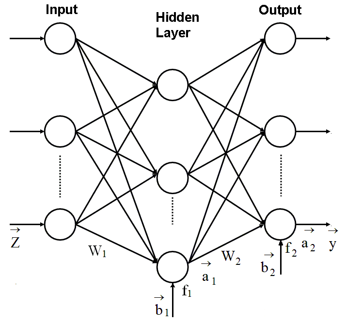
Fig. 1. Multilayer perceptron

perceptron inputs (elements of vector ) multiplied by the weight coefficients of a matrix W₁ with a bias (element of vector ) added. The neuron input is transformed by an activation function f₁ into a neuron output (element of vector ). The output layer process signals in a similar manner considering the vector as an input vector. Thus, signal processing in the perceptron is expressed as . Each output y_k is a closeness measure between the input pattern and the class D_k and the pattern is assigned to the class with a maximal closeness.

A back-propagation algorithm is usually applied for learning the MLP. In the algorithm, a network output error is propagated backwards to change unknown perceptron’s quantities W₁, , W₂ and in the direction that provides error reduction. The learning cycles repeat unless the process converges to a global error minimum. The back-propagation algorithm needs differentiable activation functions and usually they are of a sigmoid type.

The other techniques analyzed in the present paper are based on probability density estimation.

1.2. Probability density estimation

A conditional probability is a perfect criterion to classify the patterns because it minimizes classification errors and also provides a probabilistic measure of confidence to a classification decision . We can compute the probability through the Bayess formula

. (1)

If a priori information on possible faults is not available and we accept that all a priori probabilities are equal each other, probability densities are sufficient to determine a posteriori probabilities .

Since common parametric distribution functions rarely fit real distributions, let us consider nonparametric procedures. For a given point (pattern) they use nearby class patterns (learning patterns) to estimate the necessary densities. The estimation formula is simple

, (2)

where n is a total number of class patterns, V is a volume of a selected region around the point , and k is a number of learning patterns that fall into the region.

If the estimation ρ is to converge to an exact density, the quantity n should increase ensuring that

(3)

There two ways to determine V and k. The first way is to fix V and to look for k. This is a principle of the Parzen Window method. The second way is to specify k and seek for V. It is realized in the K-Nearest Neighbor method.

1.3. Parzen Windows

Different types of the region (window) for accounting the patterns are employed in the PW. For each type a specific parameter, window spread s, characterizing a region volume can be introduced.

To better describe the PW method, let us temporary assume that the region is a hypercube with a center situated at the point and length of cube edge as the spread parameter. Obviously, region volume in a m-dimensional classification space will be .

To formalize counting the patterns, let us introduce the following window function

. (4)

With this function the number of patterns inside the cube is

(5)

and the necessary density is given by

, (6)

where are training patterns. Although each window type has its own window function and spread parameter s, the function argument as well as computational equations (5) and (6) will remain the same.

Since for the given point we intend to account the nearest patterns, a hypercube is not an ideal region because the points on its surface are in a variable distance from the center. Following this logic, we can consider a hypersphere as a better choice. For a sphere window, the spread parameter is radius and the window function is expressed as

. (7)

Thus, a variation of the PW with the sphere window may have a better classification performance because of more exact density estimation according to equation (6).

As described above, for the considered cube and sphere window functions, the contribution of all inside patterns is equal to one while the outside patterns have zero contribution. Such rigid pattern separation looks like somewhat artificial. It seems more natural to assume the following rule: the closer the pattern is situated to the window center, the greater the pattern contribution will be. To realize this rule, a Gaussian window function

(8)

is usually used in the PW. The spread parameter of the Gaussian window determines its action area. To estimate probability density, the same equation (6) is employed.

On the basis of the above reasoning, we can suppose that the variation of the PW with the Gaussian window will provide the best classification performance.

The last technique to analyze and compare is the K-NN method.

1.4. K-Nearest Neighbors

All PW variations use constant window size during classification process. If actual density is low, no patterns may fall into the window resulting in zero density estimate and miss classifying. A potential remedy for this difficulty is to let the window be a function of training data. In particular, in the K-NN method we let the window grow until it captures k patterns called K-Nearest Neighbors.

The number k is set beforehand. Then for patterns of each class the sphere is determined that embraces exactly k patterns. The greater a sphere radius and volume are, the lower the density estimated by equation (2) will be.

To examine and compare the classification techniques described in this section, a special testing procedure has been developed.

2. Testing procedure

This procedure simulates a whole diagnostic process including the steps of fault simulation, feature extraction, fault classification formation, making a classification decision, and classification accuracy estimation.

2.1. Fault simulation

Within the scope of the paper, faults of engine components (compressor, turbine, combustor etc.) are simulated by means of a nonlinear gas turbine thermodynamic model

. (9)

The model compute monitored variables (temperature, pressure, rotation speed, fuel consumption, etc.) as a function of steady state operating conditions and engine health parameters . Nominal values correspond to a healthy engine whereas fault parameters imitating fault influence by shifting component performance maps.

2.2. Feature extraction

Although gas turbine monitored variables are affected by engine deterioration, the influence of the operating conditions is much more significant. To extract diagnostic information from raw measured data, a deviation (fault feature) is computed for each monitored variable as a difference between actual and baseline values. With the thermodynamic model, the deviations Z_i i=1,m induced by the fault parameters are calculated for all m monitored variables according to an expression

. (10)

A random error makes the deviation more realistic. A parameter normalizes the deviations errors resulting that they will be localized within the interval [-1,1] for all monitored variables. Such normalization simplifies fault class description.

An (m×1)-vector (feature vector) forms a diagnostic space. A value of this vector is a point in this space and a pattern to be recognized.

2.3. Fault classification formation

Numerous gas turbine faults are divided into a limited number q of classes . In the present paper, each class corresponds to varying severity faults of one engine component. The class is described by component’s fault parameters . Two class types are analyzed. A class of single faults is formed by changing one fault parameter. To create a class of multiple faults, two parameters of the same component are varied independently.

Each class is composed from numerous patterns . They are computed according to expression (10) where the necessary quantities and are generated by the uniform and Gaussian distributions accordingly. To ensure high computational precision, each class is composed from many patterns. A learning set Z1 uniting patterns of all classes presents a whole fault classification.

2.4. Making a classification decision

In addition to the given (observed) pattern and the constructed fault classification Z1, one of the chosen classification techniques is an integral part of a whole diagnostic process.

To apply and test the classification techniques, a validation set Z2 is also created in the same way as the set Z1. The difference between the sets consists in other random numbers that are generated within the same distributions.

In the considered testing procedure, an actually examined technique uses by turn one of the set Z2 patterns to set an actual point and set Z1 patterns to compute the probability densities and to make classification decision.

2.5. Classification accuracy estimation

Although the most of the considered techniques provide a confidence estimate for every pattern and classification decision (diagnosis) d_l, it is of practical interest to know classification accuracy on average for each fault class and whole engine. To this end, the testing procedure consequently applies the classification technique to all patterns of the set Z2 producing diagnoses d_l. Since true fault classes D_j are also known, probabilities of correct diagnosis (true positive rates) can be calculated for all classes resulting in a probability vector . A mean number of these probabilities characterizes accuracy of engine diagnosis by the applied technique. In the present paper, the probability is employed as a criterion to compare the techniques described in section 1.

3. Comparison conditions

For comparative calculations within the present study, a gas turbine for driving a natural gas centrifugal compressor has been chosen as a test case. It is an aeroderivative engine with a power turbine. Its thermodynamic model necessary to compute fault patterns is available. An engine operating point is close to a maximum regime and is set by a gas generator rotation speed and standard ambient conditions.

Apart from these operating conditions, the other 6 measured variables can be monitored and are used to compute patterns. These variables and their normalization parameters a_i are specified in Table 1.

Table 1

Monitored variables

№	Variable’s name	ai
1	Compressor pressure	0.015
2	Exhaust gas pressure	0.015
3	Compressor temperature	0.025
4	Exhaust gas temperature	0.015
5	Power turbine temperature	0.020
6	Fuel consumption	0.020

The faults are simulated through 9 fault parameters embedded into the model. They change from 0 to -5%. As shown in Table 2, 9 single fault classes and 4 multiple fault classes are formed. Regardless of simulated faults, single or multiple, each class is presented by n = 1000 patterns.

4. Techniques Comparison

According to the description in section 1, five classification techniques will be compared: Multilayer Perceptron (MLP), three variations of the Parzen Window method (briefly called PW-cube, PW-sphere, and PW-Gauss), and the K-Nearest Neighbor (K-NN) method. The true positive rate is a criterion to choose the best technique.

Table 2

Fault parameters and fault classes

№	Parameter names	Fault classes
		Single	Multiple
1	Compressor flow parameter	D1	D1
2	Compressor efficiency parameter	D2
3	High pressure turbine flow parameter	D3	D2
4	High pressure turbine efficiency parameter	D4
5	Power turbine flow parameter	D5	D3
6	Power turbine efficiency parameter	D6
7	Combustion chamber total pressure recovery parameter	D7	D4
8	Combustion efficiency parameter	D8
9	Inlet device total pressure recovery factor	D9

4.1. Technique adjustment

For the sake of correct comparison, each technique should be tuned to the solved problem, diagnosis of the chosen engine. The MLP was tuned for a diagnostic application in our previous works [for example, 4]. In particular, a number 27 of hidden layer nodes and a resilient back-propagation training algorithm have been found the best and were accepted for the present study.

Now, we need to tune the spread s for the variations of the PW and the nearest neighbor’s number k for the K-NN. The criterion to determine the best values of these parameters is the same, probability .

For the PW-cube technique and single fault classes, calculations with different values of the hypercube edge length s have been performed. Three groups of calculations were executed with varying seeds: with Seed 1, with Seed 2, and with 10 different seeds and averaging the probabilities . Seed means here a specific parameter that determines a series of random numbers of the used uniform and normal distributions. Figure 2 shows the resulting probabilities as a functions of the spread parameter and its optimal value s = 1.14.

Similar tuning calculations were repeated for all the techniques and two classification types. The resulting optimal values are given in Table 3. To better imagine the proportion between a window and a fault class region, remember that a maximum amplitude of pattern random errors is 1 and a total class patterns number is 1000.

One can see from the table data that the optimal spread values for the multiple faults are greater than the corresponding values of the single faults. Additionally, an optimal sphere diameters 2s is greater than the corresponding cube edges s. From our point of view,

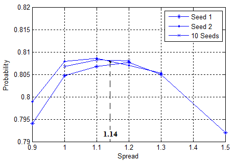
Fig. 2. Tuning the Parzen Window method

(single faults)

these facts reflect a general rule that for all cases an approximately constant proportion is conserved between the number of patterns inside the optimal window and the total number of class patterns.

Table 3

Optimal values of tuning parameters

Technique	Parameter	Classes
		Single	Multiple
PW-cube	s	1.14	1.30
PW-sphere	s	0.86	0.95
PW-Gauss	s	0.30	0.35
K-NN	k	21	18

4.2. Comparison results

With the known tuning parameter values, the calculations of the correct diagnosis probability have been executed once more by each technique and for both class types. The results are given in Table 4 where the techniques are arranged according to the probability increment. As can be seen, the PW-sphere technique is approximately equal to the PW-cube for the single faults and is more accurate for the multiple faults. In its turn, the PW-Gauss classifies fault pattern better than the PW-sphere for both class types. We can see that these conclusions about technique accuracy coincide with the suppositions made in section 1. As to the K-NN technique, it is more or less equal to the PW-Gauss: for the single faults the K-NN gains, but it yields for the multiple faults. However, these two best techniques using probability density perform worth than the MLP.

It is also can be seen that the techniques do not differ a lot: the maximum probability change within the same class type is only 0.014 (1.4%). On the other hand, it was shown in [4] that computational errors are pretty great, ±0.01. This means that the differences between the techniques can be partly explained by low computational precision.

Table 4

Probabilities for different techniques

Technique	Classes
	Single	Multiple
PW-cube	0.8101	0.8648
PW-sphere	0.8098	0.8698
PW-Gauss	0.8131	0.8748
K-NN	0.8160	0.8720
MLP	0.8238	0.8760

Preliminary, we can state that the PW-Gauss and K-NN techniques do not yield a lot to the MLP. Because these two classification techniques have an advantage of providing a confidence measure for every classification decision, they can be recommended for real application.

Discussion

The present paper can be considered only as a preliminary study. In spite of some results obtained, the paper revealed important issues to be solved in future.

First, to draw final conclusion on techniques efficiency, the comparative calculations should be repeated with higher precision. We find it possible to decrease computational errors in 10 times.

Second, since estimating diagnostic decision confidence is an important property of the analyzed techniques, it seems to be of practical interest to determine the estimation precision.

Third, in the present study, the techniques were examined at one static gas turbine operating point i.e. for one-point diagnosis. Because multipoint diagnosis and diagnosis at transients promise more accurate results, it seems important to examine the techniques for these perspective diagnostic options.

Conclusions

Thus, in the present paper four techniques have been examined that classify gas turbine faults through estimating probability densities for the considered classes. They were compared with each other and with the Multilayer Perceptron (MLP) using the criterion of mean probability of correct diagnosis. It was found that the best two techniques, Parzen Windows with Gaussian window and K-Nearest Neighbors, yield just a little to the MLP. These two techniques are recommended for gas turbine diagnosis because they provide confidence estimation for each diagnostic decision, the property very valuable in practice.

The present study also revealed some issues to solve in future investigations. They are related with more precise probability computation and with study extension on multipoint and transient diagnosis.

Acknowledgments

The work has been carried out with the support of the National Polytechnic Institute of Mexico (research project 20131509).

References

1. Roemer M. J. Advanced diagnostics and prognostics for gas turbine engine risk assessment [Text] / M. J. Roemer and G. J. Kacprzynski // Proc. ASME Turbo Expo 2000, Munich, Germany, May 8-11, 2000. − 10p.

2. Ogaji S.O.T. Gas path fault diagnosis of a turbofan engine from transient data using artificial neural networks [Text] / S.O.T. Ogaji, Y. G. Li, S. Sampath, et al. // Proc. ASME Turbo Expo 2003, Atlanta, Georgia, USA, June 16-19, 2003. − 10p.

3. Volponi A.J. The use of Kalman filter and neural network methodologies in gas turbine performance diagnostics: a comparative study [Text] / A.J. Volponi, H. DePold, R. Ganguli // Journal of Engineering for Gas Turbines and Power. − 2003. − Vol. 125, Issue 4. − P. 917-924.

4. Loboda I. Neural networks for gas turbine fault identification: multilayer perceptron or radial basis network [Text] / I. Loboda, Ya. Feldshteyn, V. Ponomaryov // International Journal of Turbo & Jet Engines. − 2012. − Vol.29, Is. 1. − P. 37-48 (ASME Paper No. GT2011-46752).

5. Loboda I. On the selection of an optimal pattern recognition technique for gas turbine diagnosis [Text] / I. Loboda, S. Yepifanov // Proc. ASME Turbo Expo 2013, San Antonio, Texas, USA, June 3-7, 2013. − 11p., ASME Paper No. GT2013-95198.

6. Duda, R.O. Pattern Classification [Text] / R.O. Duda, P.E. Hart, D.G. Stork. − New York: Wiley-Interscience, 2001. − 654 p.