Probabilistic Neural Networks For Gas Turbine Fault Recognition
Gas turbine fault isolation or identification generally uses a model-based classification of gas path faults. This classification is not too exact because of model errors. The present paper looks at the possibility to create a fault class on the basis of gas turbine real data containing cycles of a compressor fouling and washing. The concerned data-driven fouling class formation is realized in the space of deviations of measured gas path quantities. Analyzing deviation plots for different fouling cycles, we have confirmed identifiability of the fouling. In order to draw sound conclusions, the analysis was conducted for two gas turbines of different application.
Gas turbine, field data, compressor fouling, deviations of measured variables
1. Introduction
In modern gas turbine health monitoring systems, the algorithms of fault identification based on treatment of gas path measured quantities (pressures, temperatures, rotation speeds, fuel consumption, etc.) are considered as principal and sufficiently complex techniques [see, for example, 1]. These algorithms are capable to identify (isolate) such gas turbine performance deterioration (degradation) mechanisms as fouling, tip rubs, seal wear, and erosion in different gas path components e.g. compressors, turbines, and a combustor. The degradation mechanisms (let’s call them faults) evolve gradually over the long time of operation and induce increasing deviations of measured gas path variables. Above these gas path faults, measurement system malfunctions can also be isolated on the measured quantities [2].
To build a classification required for fault identification, various gas path mathematical models are widely used [see 2 and 3] because of high cost of physical simulation of the degradation mechanisms and infrequent fault displays. In this case, model errors are transmitted to the model-based classification and the problem arises to make the fault classification more exact using real data. Moreover, the necessary model can not sometimes be available and real data on fault displays can be unique information to build the classification.
It is famous that the most common cause of stationary gas turbines’ deterioration is a compressor fouling. The impact of the fouling on gas turbine performance is well described [4,5] and data with fouling and washing cycles are widely used in order to verify diagnostic techniques [see, for example, 6 and 7].
In the previous papers [8,9], we also involved maintenance data (field data) with influence of the fouling into diagnostic analysis. Deviations of measured quantities from their baseline (reference) values were employed as fouling indicators. The analysis objective was to ensure high quality of the deviations by detecting measurement errors, extracting them from analyzed data, and enhancement of a baseline function. Possible error sources were examined and some methods were proposed to compute this function.
Proceeding with our work on field data with fouling and washing cycles, the present paper looks at the deviations as patterns to construct a data-driven class of the fouling. It is supposed to incorporate this class into the fault classification for gas turbine diagnostics instead a model-based fouling class. The objective of the paper is to verify whether the fouling can be well identifiable on the background of other degradation mechanisms. To that end, we study its properties by means of analyzing numerous 2D and 3D deviation plots. In section 2, the analysis is performed on field data of two industrial gas turbines and in section 3 field and model data are compared.
2. Fouling Analysis on Real Data
2.1. Approach Applied
A deviation calculation is an important preliminary operation before the stages of gas turbine monitoring, diagnostics, and prognostics. A relative deviation
![]() of a measured gas path variable
of a measured gas path variable
![]() can be computed as
can be computed as
 , (1)
, (1)
where
![]() is a baseline function, which corresponds to a healthy engine. The function’s arguments united in a vector
is a baseline function, which corresponds to a healthy engine. The function’s arguments united in a vector
![]() are atmospheric conditions and engine control variables known all together as operating conditions. The deviations
are atmospheric conditions and engine control variables known all together as operating conditions. The deviations
![]() computed for all monitored variables are mostly free of the influence of operating conditions and can be good engine performance deterioration indicators.
computed for all monitored variables are mostly free of the influence of operating conditions and can be good engine performance deterioration indicators.
A deviation value always contains random errors caused by measurement inaccuracy and baseline function uncertainty. Being great, these errors can mask the deterioration effect, in particular, the fouling influence. Hence, it is of great importance to reduce the errors and make the fouling more identifiable.
Let’s denote the highest possible random error in deviation (1) by
![]() and calculate a normalized deviation
and calculate a normalized deviation
 . (2)
. (2)
As maximum error of each normalized deviations is equal to one, the fault class description will be uniform for all monitored variables. That is why in the present paper, the fouling class is described and analyzed in the diagnostic space of the deviations (2). The normalized deviations of all monitored variables computed for one measurement time section compose the vector that is a point in the diagnostic space and a pattern to be recognized. Every fault class including the fouling class is presented by a set of patterns.
During the computing the deviations, it is a main problem to get an adequate baseline function. Polynomials and artificial neural networks are usually applied to that end and a learning set of real data is used to identify them. We showed in previous works [8,9] that the second order full polynomials adequately describe behaviour of a healthy engine. We also revealed that the learning set generated by a gas turbine thermodynamic model permits to get a good baseline function. That is why the second order polynomials and the thermodynamic model are employed in the present paper. In addition to generating the learning set, this model is applied for simulating the compressor fouling.
The model has the following structure
![]() (3)
(3)
and relates the gas path variables with the operating conditions and fault parameters
![]() . These parameters are used to displace performance maps of engine components and simulate different faults in this way.
. These parameters are used to displace performance maps of engine components and simulate different faults in this way.
In the present paper, fouling analysis on real data will be carried out in the space of the deviations by plotting data with different fouling cycles and by the visual examination of suitability of the plotted data for construction of a representative fouling class. In particular, the properties will be verified of (a) deviation sensibility to the fouling, (b) low deviation errors, (c) uniform pattern distribution in the fouling class area, and (d) repeatability of the class area for various fouling cycles.
Two following subsections deal with the data analysis for two free turbine power plants of different application. The first of them called in this paper as Engine 1 drives a centrifugal compressor in natural gas pipelines, while the second called Engine 2 is a driver of an electrical generator. During prolonged periods of time, field data of these engines were registered in special diagnostic databases within an hour interval. The data cover numerous cycles of the fouling and washing. Our preliminary analysis shows that engines’ performances are recovered after the washings. That is why the fouling can be considered as a unique degradation mechanism affecting the engines during the registration periods.
2.2. Engine 1 Data Analysis
For Engine 1, a total registration period embraces 2605 hours of operation and consists of two intervals of the fouling with the washing between them. The washing takes place after the 1010th hour of operation.
As described before, the chosen baseline function presents the second order full polynomial. To introduce engine operating conditions into the function, four arguments have been selected for Engine 1: fuel consumption, free turbine (power turbine) rotation speed, inlet temperature, and atmospheric pressure. These arguments almost completely determine an engine operating point and ensure the smallest deviation errors. To calculate polynomial’s coefficients, the data generated by the thermodynamic model of type (3) was employed.
On the basis of the calculated baseline functions, deviations (1) have been computed for all monitored gas path variables. As a result of analyzing and comparing deviation plots, four most informative deviations were selected for further analysis and their highest possible errors were estimated. Table 1 specifies the deviations and their error parameters.
Table 1. Deviations analyzed for Engine 1.
Deviation notation |
Name of monitored variable |
Error |
dTt |
High pressure turbine temperature |
0.0050 |
dTpt |
Power turbine temperature |
0.0060 |
dPt |
High pressure turbine pressure |
0.0055 |
dPc |
Compressor pressure |
0.0090 |
Note: The name of variable references to an outlet section of the corresponding engine component.
In Fig.1, time plots of the selected deviations are presented. As can be seen for all deviations, an influence of the fouling and washing is clearly visible in the background of random fluctuations. However, gas turbine faults are usually identified and a fault classification is constructed in the multidimensional space of normalized deviations (2). For this reason, we also plotted 3D and 2D diagrams of normalized deviations (patterns) without a time variable.
Figure 2 shows the 3D diagram for the first three variables of Table 1. Patterns of the first and the second fouling intervals are marked here and below as F1 and F2 correspondingly. As one 3D diagram does not give a full picture of a pattern distribution, three projections are also given in Fig.3.
It can be seen in the both figures that the fouling patterns create a compact and elongated areas. This means that the chosen deviations are sensible to the fouling and the deviation errors are relatively small. In other words, the signal-to-noise ratio is relatively great. It can additionally be stated that the pattern areas of two fouling intervals are pulled out in the same direction, namely the fouling influence on the monitored variables does not change with the gas turbine operation time.
Engine 2 data are also attracted in order to generalize the analysis and conclusions. For this engine, the fouling analysis is conducted in the next subsection in the same manner as for Engine 1.
2.3. Engine 2 Data Analysis
A total period of Engine 2 field data registration includes 4914 hours of operation and consists of five intervals of the fouling with the washings at the time points t = 803, 1916, 3098, and 4317.
For the need of an electrical generator, a free turbine rotation speed is maintained constant. Therefore, the baseline function has only three arguments. The chosen arguments that ensure the smallest deviation errors are free turbine power, atmospheric temperature, and inlet pressure.
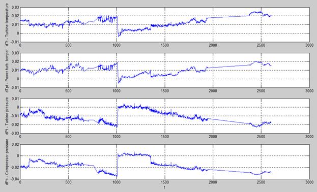
Fig.1. Time plots of Engine 1 deviations.
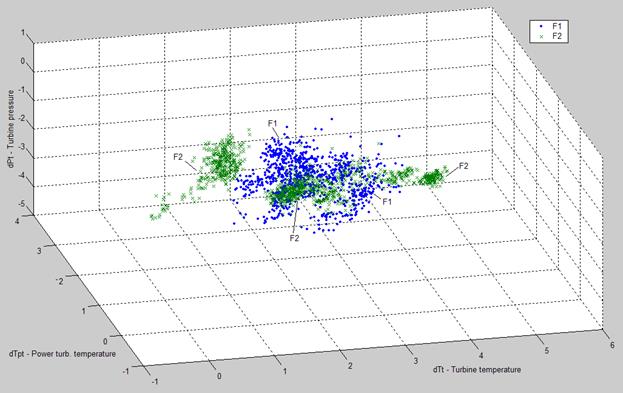
Fig.2. 3D diagram of Engine 1 normalized deviations.
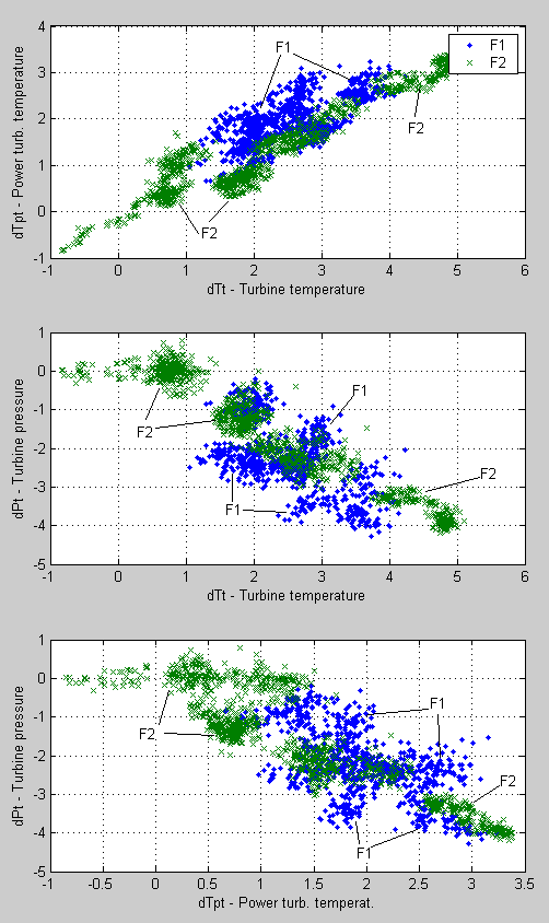
Fig.3. 2D diagrams of Engine 1 normalized deviations.
A thermodynamic model was not available for Engine 2 and a learning set for computing baseline function coefficients was composed from field data.
Only three deviations were found to be informative for the considered engine. These deviations and their errors are specified in Table 2.
Table 2. Deviations analyzed for Engine 2.
Deviation notation |
Name of monitored variable |
Error |
dTc |
Compressor temperature |
0.0080 |
dTt |
High pressure turbine temperature |
0.0060 |
dTpt |
Power turbine temperature |
0.0110 |
Figure 4 shows time plots of the selected deviations. One can see that an influence of the fouling and washing is as clearly visible as in the case of Engine 1.
In figures 5 and 6, the 3D diagram and the projection graphs are presented. The fouling interval are marked here as F1, F2, …, F5. As can be seen in the figures, the distribution of Engine 2 patterns confirms the conclusions drawn for Engine 1: the deviations are sensible to the fouling, the errors are relatively small, the patterns are uniformly distributed, and the fouling influence on the deviations is the same for all five intervals.
Availability of the Engine 1 thermodynamic model allows comparing real fouling displays with simulated data.
3. Comparison of Real and Simulated Engine 1 Fouling Data
Software of the thermodynamic model permits to calculate a linear model
![]() , (4)
, (4)
which connects small changes of fault parameters
![]() and gas path variables
and gas path variables
![]() by an influence matrix H for fixed operating conditions.
by an influence matrix H for fixed operating conditions.
This linear model was used in the presented analysis on order to simplify the fouling simulation by calculating numerous patterns.
To conserve fouling influence, the engine operating point for calculating the influence matrix was given by the fixed values of the same variables that were used in subsection 2.2 as the arguments of a baseline function. The fouling was simulated by gradual changes
![]() and
and
![]() of the compressor fault parameters, compressor flow decrease and compressor efficiency decrease, from zero to their minimal values - 0.030 and - 0.015. The deviations
of the compressor fault parameters, compressor flow decrease and compressor efficiency decrease, from zero to their minimal values - 0.030 and - 0.015. The deviations
![]() induced by
induced by
![]() and
and
![]() were normalized then. In order to estimate the model accuracy, the normalized simulated deviations with and without errors were finally compared with real fouling data.
were normalized then. In order to estimate the model accuracy, the normalized simulated deviations with and without errors were finally compared with real fouling data.
With the purpose of better comparison, the model-based deviations and data-driven ones are plotted together in common coordinates. Two 3D diagrams are presented in figures 7 and 8. In Fig.7, simulated deviations without errors are given in the plane that is parallel to the line of fouling severity increase while Fig.8 presents a transversal view where the simulated fouling is projected to a point. The simulated data are marked here and below by “M”-letter.
In figures 9 and 10, 2D graphs are presented. Figure 9 illustrates the case of simulated data without errors and in Fig. 10 the data with errors are shown. It can generally be concluded from observing all plots that the thermodynamic model correctly reflects the fouling influence on monitored variables despite of a slight displacement of simulated data.
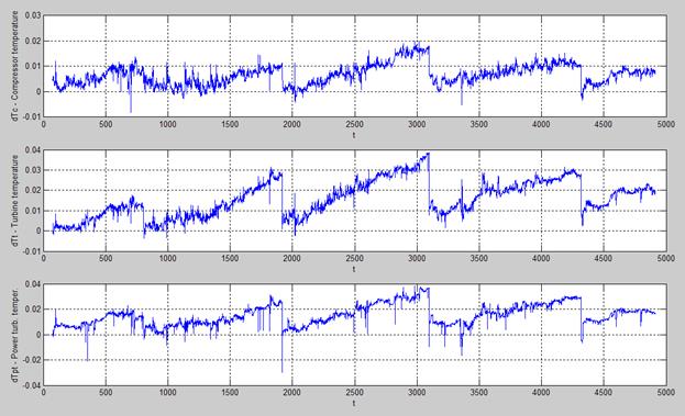
Fig.4. Time plots of Engine 2 deviations.
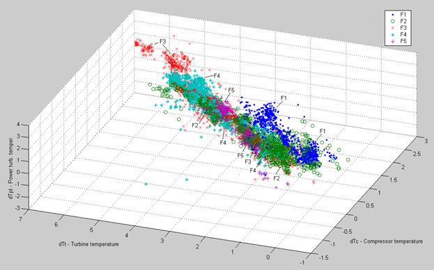
Fig.5. 3D diagram of Engine 2 normalized deviations.
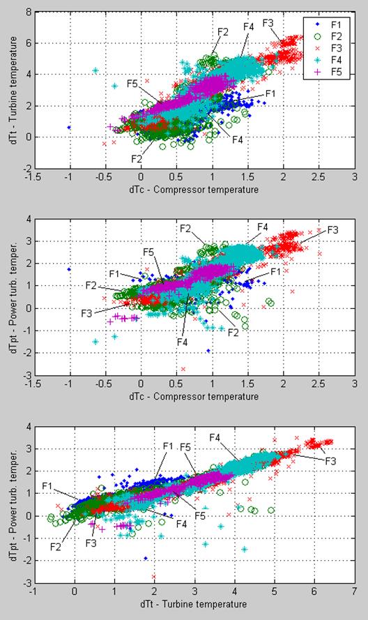
Fig.6. 2D diagrams of Engine 1 normalized deviations.
Conclusions
Thus, analyzing deviation plots based on real gas turbine data, we have demonstrated the possibility to create well recognizable class of compressor fouling. The deviations were found to be sensible to the fouling and a class area was compact and time stable. To better study the foiling class’ properties, the analysis was performed on field data of two different gas turbines.
Comparing real and simulated data of one of the analyzed gas turbines, we have also shown that the thermodynamic model satisfactorily describes the fouling influence on gas turbine performance.
The above conclusions support the idea of a mixed fault classification that incorporates both model-based and data-driven fault classes. Such a classification will combine a profound common diagnosis with an elevated diagnostic accuracy for the data-driven classes.
The present paper can be considered only as the first attempt to analyze data-driven fault classes. Visual qualitative analysis will be accompanied by quantitative estimations of class properties in our future works.
Acknowledgments
The work has been carried out with the support of the National Polytechnic Institute of Mexico (project 20080974).
References
1. Boyce, Meherwan P. Gas Turbine Engineering Handbook.- Gulf Publishing Company.- 1995.
2. C. Romesis, K. Mathioudakis. Setting up of a probabilistic neural network for sensor fault detection including operation with component fault// Journal of Engineering for Gas Turbines and Power. 125.- 2003.- pp. 634-641.
3. Roemer M.J., Kacprzynski G.J. Advanced diagnostics and prognostics for gas turbine engine risk assessment// Proc. ASME Turbo Expo Conf., Germany.- 2000.- 10p.
4. Saravanamuttoo H.I.H., MacIsaac B.D. Thermodynamic models for pipeline gas turbine diagnostics// ASME Journal of Engineering for Power. 105.- 1983.- pp.875-884.
5. Tarabrin A. P., Schurovsky V. A., Bodrov A. I., Stalder J. –P. An analysis of axial compressor fouling and a blade cleaning method// ASME Journal of Turbomachinery. 120.- 1998.- pp. 256 – 261.
6. Kacprzynski Gregory J. et al. A prognostic modelling approach for predicting recurring maintenance for shipboard propulsion system. Proc. ASME Turbo Expo Conf., USA.- 2001.- 7p.
7. Bryce Lord, Joshua Bennett. Equipment health monitoring failure mode characteristics case study// Proc. 17th National Petroleum Show, Canada.– 2000.- 25p.
8. Julio César Hernández González, Igor Loboda, Carlos de la Cruz Alejo. Development of normal state model for gas turbine performance monitoring // Memorias del 3er Congreso Internacional de Ingeniería Electromecánica y de Sistemas, México.- 2002, pp. 243 – 246.
9. Loboda I., Yepifanov S., Feldshteyn Y. Deviation problem in gas turbine health monitoring// Proc. IASTED International Conference on Power and Energy Systems, USA.- 2004.- 6p.
Поступила в редакцию 01.08.08
Рецензент: канд. техн. наук, профессор Гусев Ю. А., Национальный аэрокосмический университет им. Жуковского «ХАИ», Харьков.
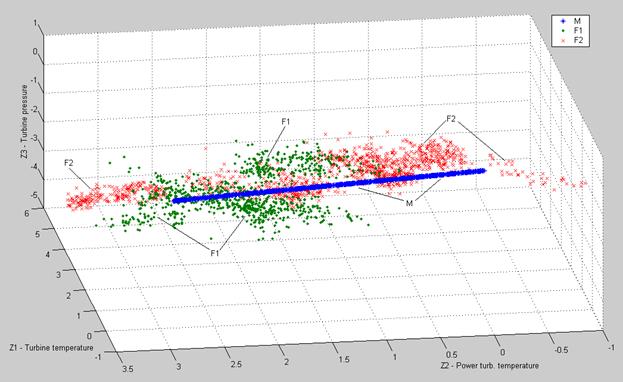
Fig.7. 3D diagram of Engine 1 real and simulated fouling data (longitudinal view).
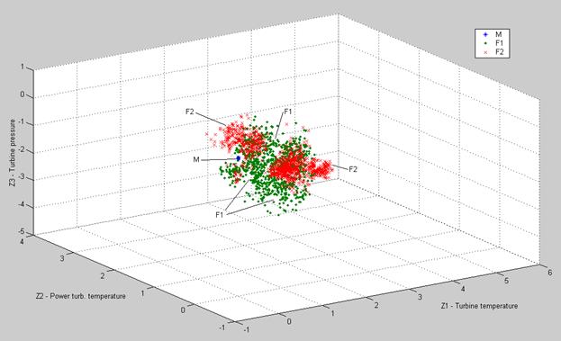
Fig.8. 3D diagram of Engine 1 real and simulated fouling data (transversal view).
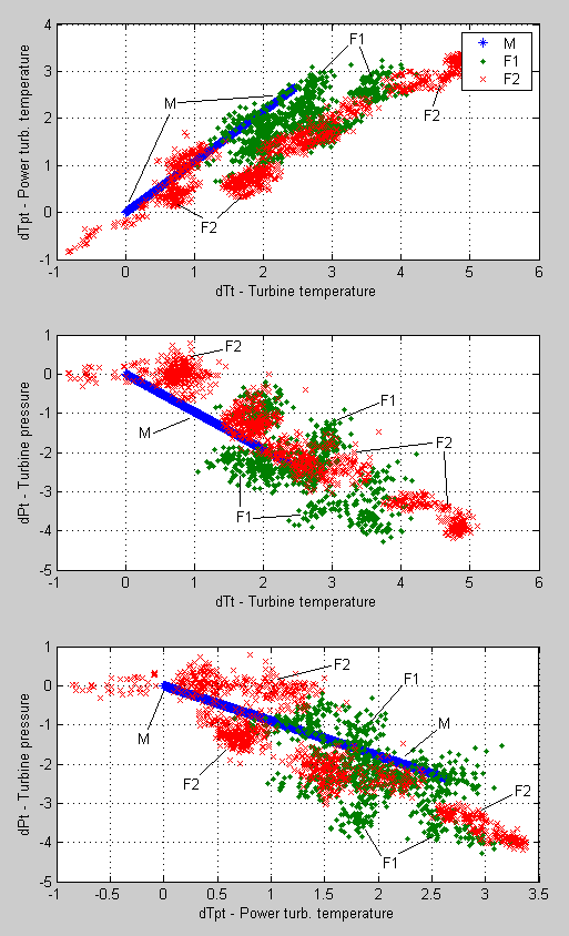
Fig.9. 2D diagrams of Engine 1 real fouling data and results of the deviations simulation without errors.
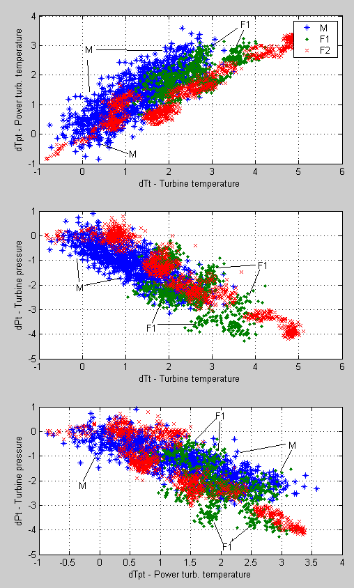
Fig.10. 2D diagrams of Engine 1 real fouling data and results of the deviations simulation with errors.